Modeling and simulation of convection-dominated species transfer at rising bubbles
Andre Weiner, weiner@mma.tu-darmstadt.de
First supervisor: Prof. Dr. rer. nat. Dieter Bothe
Second supervisor: Prof. Dr.-Ing. Peter Stephan
Gas-liquid reactors
micro reactor
size: millimeter
source: SPP 1740
prediction of
- mass transfer
- enhancement
- mixing
- conversion
- selectivity
- yield
- ...
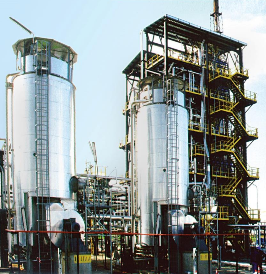
bubble column reactor
size: meter
source: R. M. Raimundo, ENI
High Péclet number problem
U. D. Kück, M. Schlüter, N. Räbiger:
Analyse des grenzschichtnahen Stofftransports an frei aufsteigenden Gasblasen (2009)
Specimen calculation
$d_b=1~mm$ water/oxygen at room temperature
- $Pe = Sc\ Re = \nu_l / D_{O_2} \cdot U_b d_b/\nu_l \approx 10^5 $
- $$ Re\approx 250;\quad \delta_h/d_b \propto Re^{-1/2};\quad\delta_h\approx 45~\mu m $$
- $$ Sc\approx 500;\quad \delta_c/\delta_h \propto Sc^{-1/2};\quad\delta_c\approx 2.5~\mu m $$
$\delta_h/\delta_c$ typically 10 ... 100
feasible simulations up to $Pe\approx 1000$ (3D, HPC)
Outline
- Effect of underresolved meshes
- Subgrid-scale modeling
- Data-driven modeling
- Subgrid-scale model assessment
- Comparison with experiments
- Summary and outlook
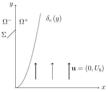
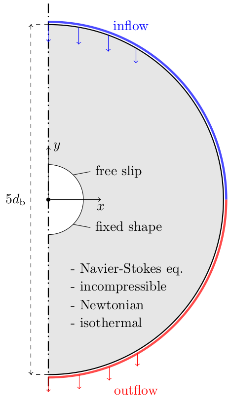
Underresolved meshes
- $c_A|_\Sigma = const.$
- $\mathbf{u}$ - given velocity vector field
- finite volume discretization
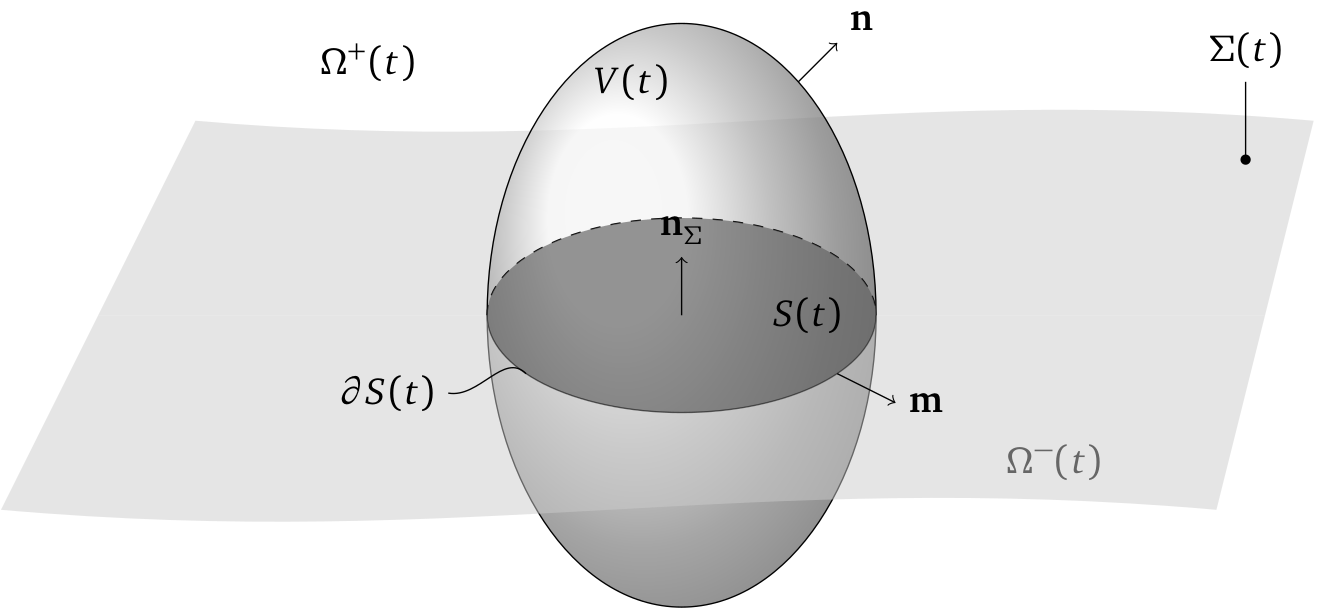
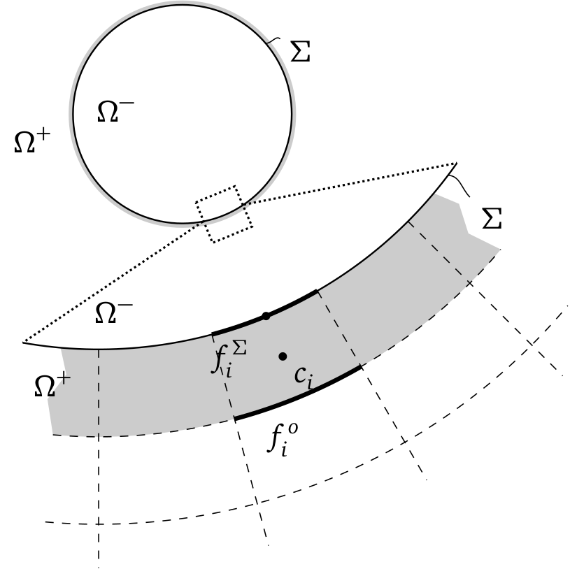 $\Omega^\pm$ - liquid/gas domain, $\Sigma$ - interface, $f_i$ - cell faces
Transfer species - A
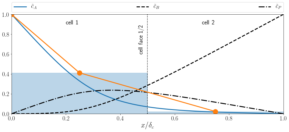 Normalized concentration profile $\tilde{c}_A$ in interface normal direction $x/\delta_c$ for the transfer species (solid blue line),
average concentration values per cell (shaded blue), and linear reconstruction (orange).
Normalized concentration profile $\tilde{c}_A$ in interface normal direction $x/\delta_c$ for the transfer species (solid blue line),
average concentration values per cell (shaded blue), and linear reconstruction (orange).
Interpolation errors
Subgrid-scale modeling
Idea: Leverage coherent structures in convection-dominated species boundary layers.
-
Substitute problem
Find a representative substitute problem to obtain a parameterized profile function. -
Reconstruction
Adjust the profile function based on local simulation data (cell-width, average concentration, ...). -
Correction
Correct convective fluxes, diffusive fluxes, and reaction source terms based on the adjusted profile function.
(1) Substitute problem
$$ \partial_\tilde{y} \tilde{c} = \frac{1}{Pe}\partial_{\tilde{x}\tilde{x}} \tilde{c}$$
- $\tilde{c}(\tilde{x}=0,\tilde{y}) = 1$
- $\tilde{c}(\tilde{x}>0,\tilde{y}=0) = 0$
- $\tilde{c}(\tilde{x}\rightarrow\infty,\tilde{y}) = 0$
- 2004 - first idea, physisorption
- 2010 - first implementation by Alke, Bothe, Kröger, Weigand, Weirich and Weking
- 2013 - improved implementation by Bothe and Fleckenstein
- 2016 - extension to first order reaction by Gründing, Fleckenstein and Bothe
(2.1) Reconstruction
(3.1) Correction
-
compute interface normal derivative:
$\partial_\tilde{x} \tilde{c}|_{\tilde{x}=0} = 2/(\sqrt{\pi}\delta_{num})$ - correct numerical diffusive flux at $\tilde{x}=0$
- solve transport equation for $\tilde{c}$
→ saves one refinement level (half cell-width)
A Volume-of-Fluid-based method for mass transfer processes at fluid particles (2013)
(3.2) Correction
Correct convective and diffusive fluxes over all cell faces of an interface cell.
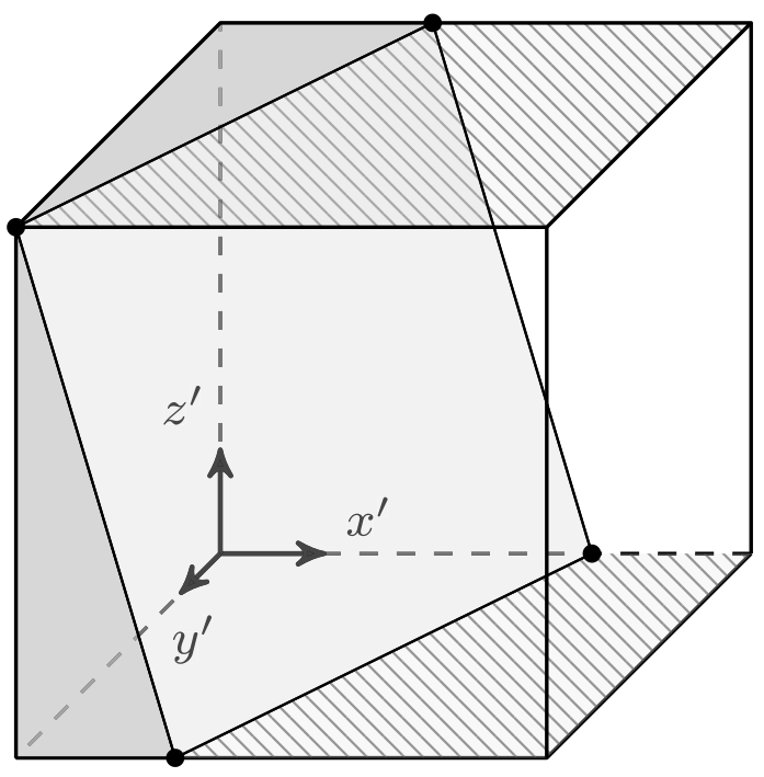 Control volume (cube) with embedded interface (plane).
(2.2) Reconstruction
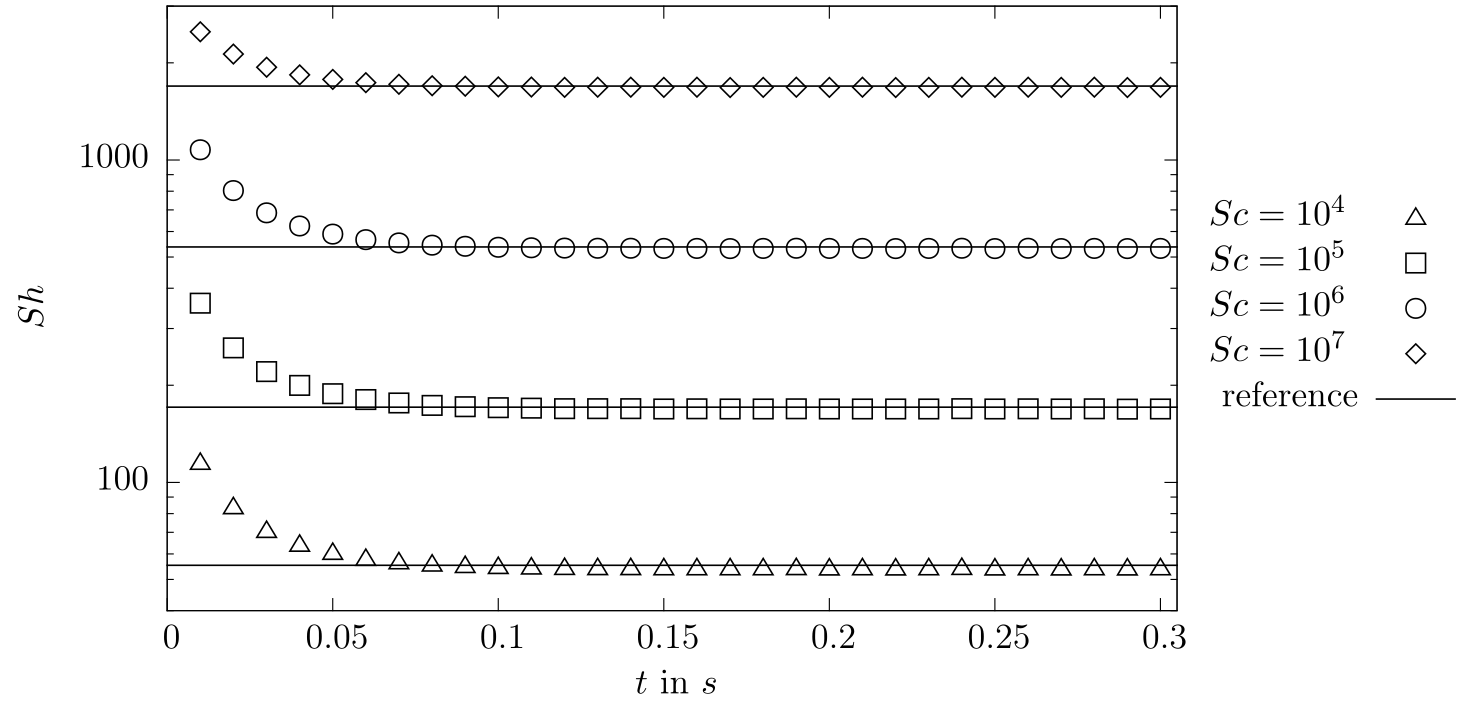
Results
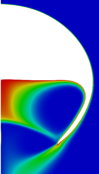
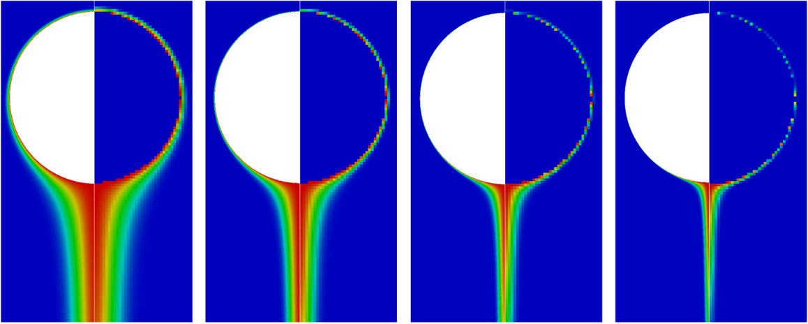 Normalized concentration field of Stokes-flow reference solution (left half) and subgrid-scale solution (right half) for $Sc=\nu/D=10^4/10^5/10^6/10^7$ (left to right).
Results
$Sh = \frac{k_L d_b}{D}$ with $k_L = \frac{\dot{N}}{A_{eff}\Delta c}$
Data-driven modeling
Idea: Replace analytical solution with machine learning (ML) model.
-
Substitute problem
Find a representative substitute problem and solve it numerically to obtain boundary layer data. -
Model creation
Select meaningful features (variables) and train a ML model. -
Correction
Correct convective fluxes, diffusive fluxes, and reaction source terms based on the ML model.
ML terminology
$s$ instances of feature - label pairs
| $s$ | $x_{1,s}$ | $x_{2,s}$ | $x_{3,s}$ | $y_s$ |
|---|---|---|---|---|
| 1 | 0.1 | 0.4 | 0.6 | 0.5 |
| 2 | ... | ... | ... | ... |
prediction
error norm
$\hat{y}_s = f_m(x_{1,s}, x_{2,s}, x_{3,s})$
$L_i = L_i(y_s - \hat{y}_s)$
(1) Substitute problem
numerical solution
- OpenFOAM®
- steady-state flow dynamics
- parameters: $Re$, $Sc_i$, $Da_i$, shape, ...
- finished in minutes
data extraction
- features (input variables) should be available in target simulation
- features motivated by boundary layer theory and previous modeling
- down-sampling to coarse meshes
- stored as comma separated values (csv)
(2) Model creation
Multilayer Perceptron
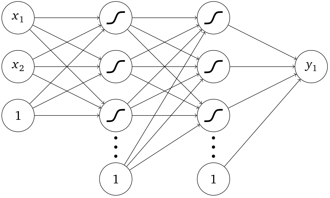
- 6 layers with 40 neurons per layer
- SELU activation function
model training
- mean squared error loss
- one model per label
- ≈ 5 min training time per model
- training on CPU with double precision
implementation
- PyTorch®
- export to TorchScript
- dynamically loaded at runtime
SGS Model assessment
Aim:
Create reference data for complex shapes and flow scenarios to assess model generalization.
Idea:
Decoupling of two-phase flow and species transport.
1. Two-phase flow simulation (Volume-of-Fluid)
2. Parametrization of shape and interfacial velocity
3. Geometry generation and export (STL format)
4. Single phase mesh
5. Flow solution
6. Species transport
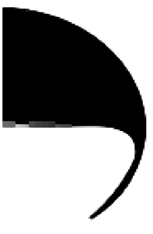
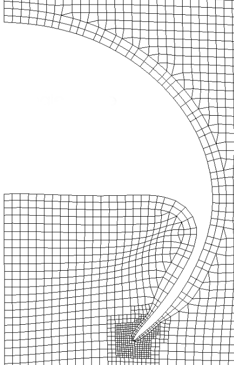
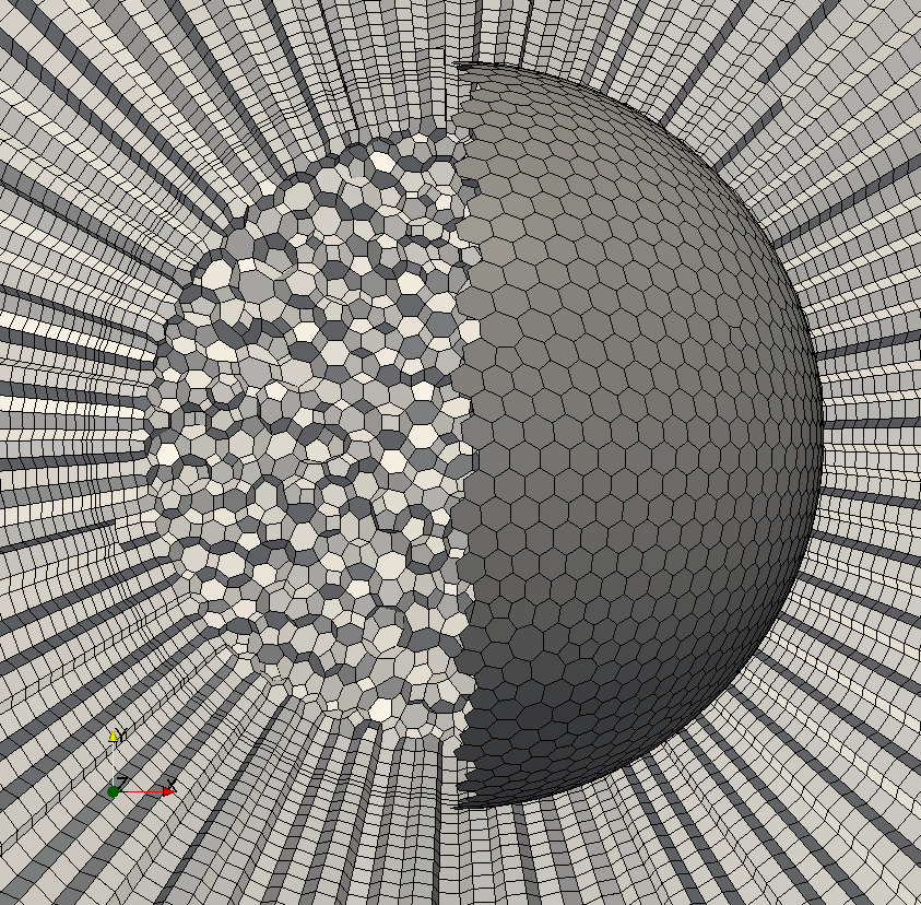
Mesh dependency
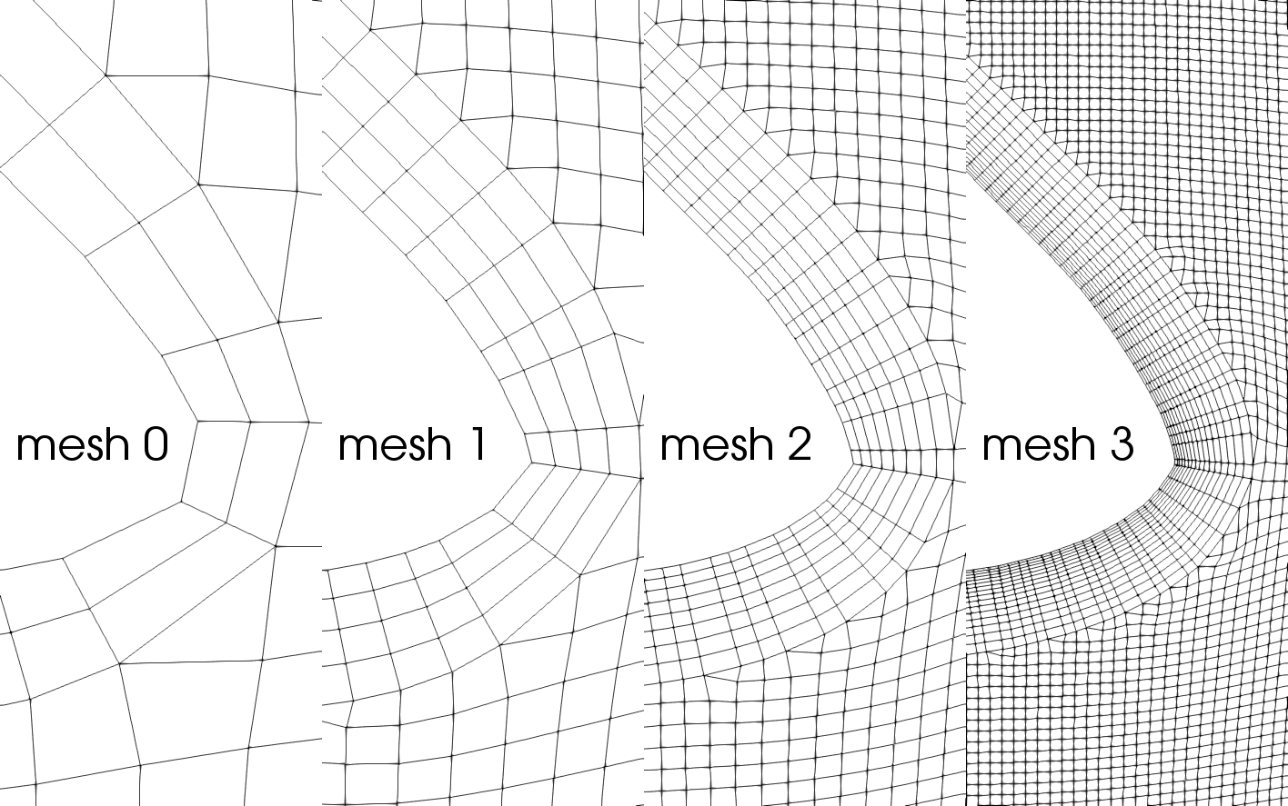
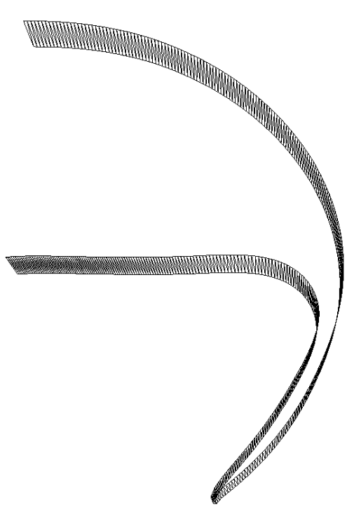
Prismatic cell layers around a spherical-cap bubble with increasing mesh resolution.
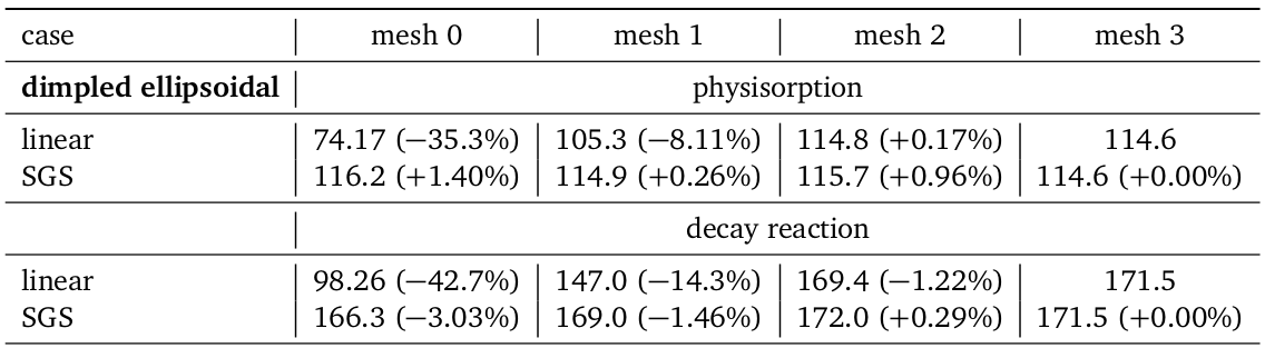
Model assessment
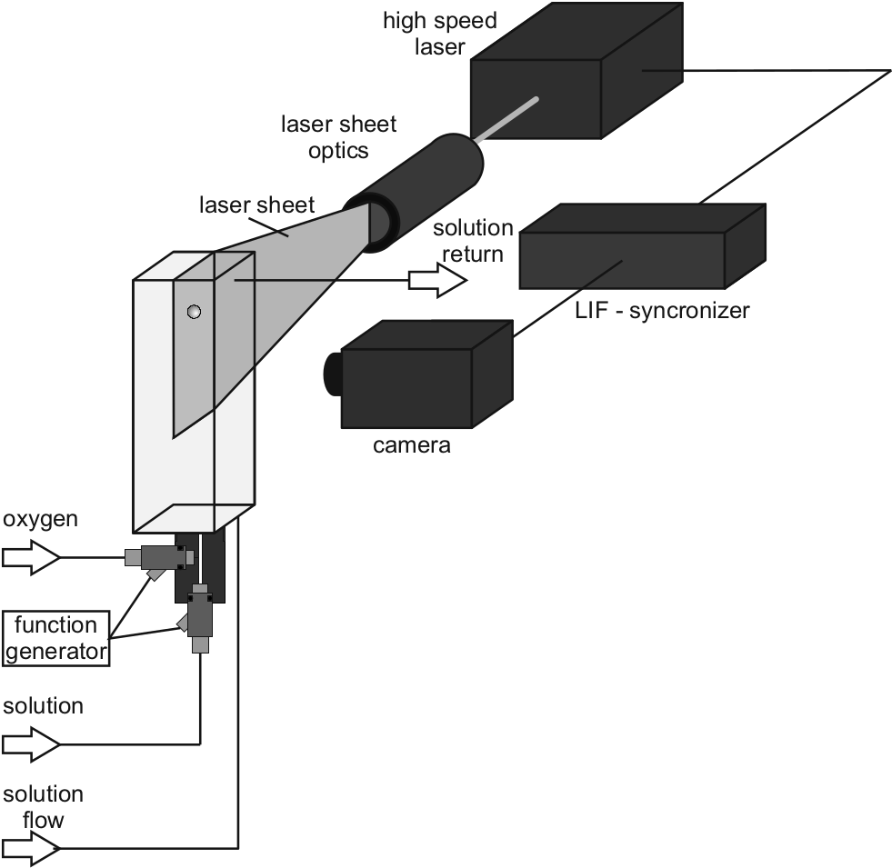
Comparison with experiments
Mathematical model
Interface Tracking
- numerical equivalent of sharp interface model
-
surface tension isotherms
$\sigma = \sigma (c^\Sigma)$ - sorption library $ s^\Sigma + [\![ -D\nabla c ]\!]\cdot \mathbf{n}_\Sigma = 0$
- here: Langmuir fast sorption model
Computational analysis of single rising bubbles influenced by soluble surfactant (2018)
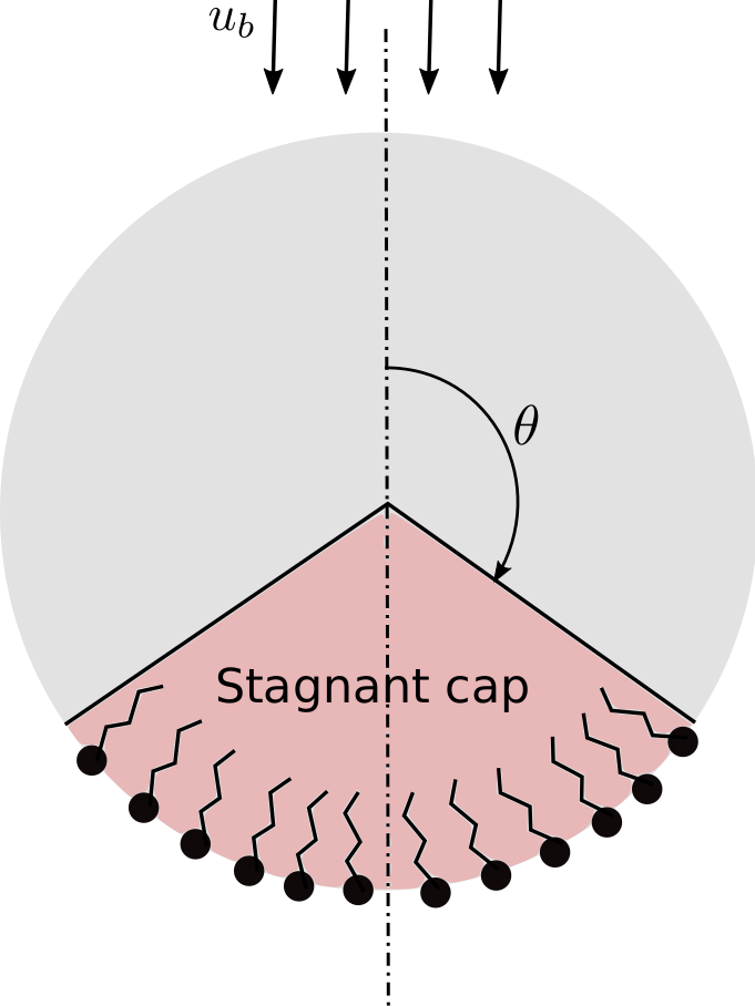 Surfactant - surface active agent
Velocity
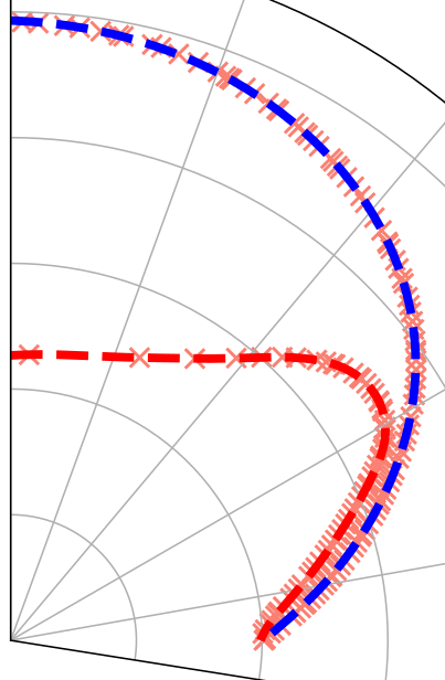
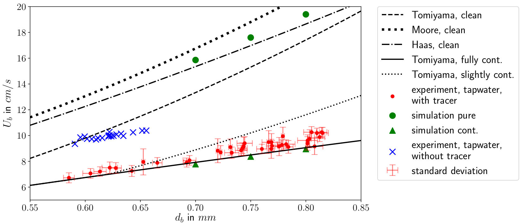 Terminal velocity plotted against the bubble diameter. Experimental, numerical, theoretical and literature results.
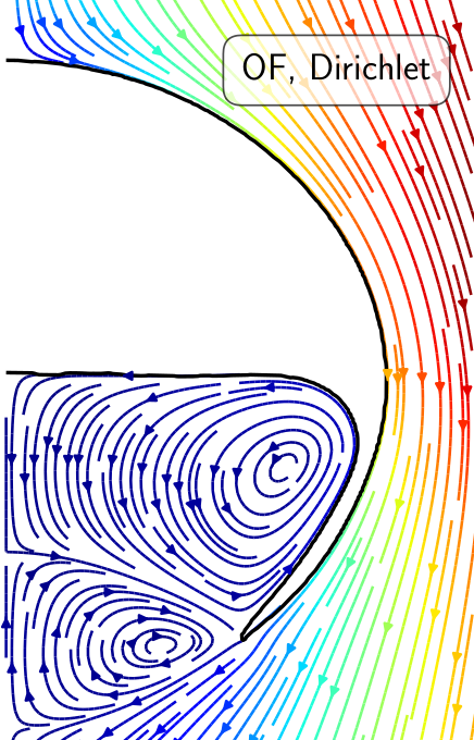
Local velocity
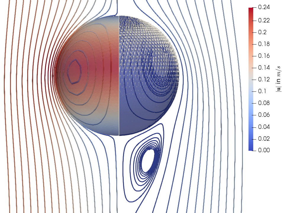 Streamlines and magnitude of interfacial velocity for clean (left) and contaminated (right) interfaces. The glyphs depict local Marangoni forces.
Oxygen transport
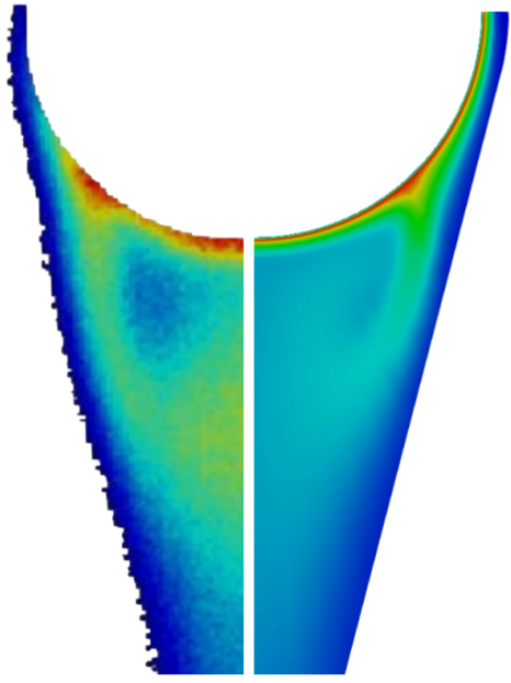
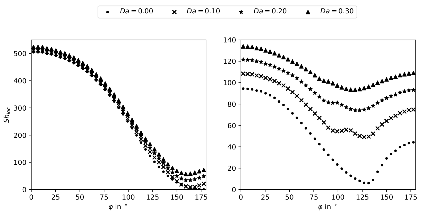 Local Sherwood number for clean (left) and contaminated (right) interfaces.
Experimental and numerical investigation of reactive species transport around a small rising bubble (2019)
Summary
- high-$Pe$ number problem (boundary layer)
- influence on numerical solution
- SGS modeling for complex reactions
- hybrid approach for high-fidelity reference data
- validation with complex bubble shapes
- qualitative and quantitative agreement with experiments
- new understanding of dynamic surfactant adsorption
- well documented, fully reproducible, public research results and methods
- pathway paved for data-driven solutions in computational fluid dynamics
Outlook
- (data-driven) modeling for the liquid bulk
- assessment for dynamic interfaces
- application to related boundary layer problems
THE END
Special thanks to David Merker, Jens Timmermann, Chiara Pesci and Dennis Hillenbrand
Thank you for your attention!
Get in touch: weiner@mma.tu-darmstadt.de
Complementary material
Publications
Advanced subgrid-scale modeling for convection-dominated species transport at fluid interfaces with application to mass transfer from rising bubbles, J. Comput. Phys. (2017)
Computational analysis of single rising bubbles influenced by soluble surfactant, J. Fluid Mech., (2018)
Experimental and numerical investigation of reactive species transport around a small rising bubble, Chem. Eng. Sci., (2019)
Data‐Driven Subgrid‐Scale Modeling for Convection‐Dominated Concentration Boundary Layers, Chem. Eng. and Techn. (2019)
Reproducibility
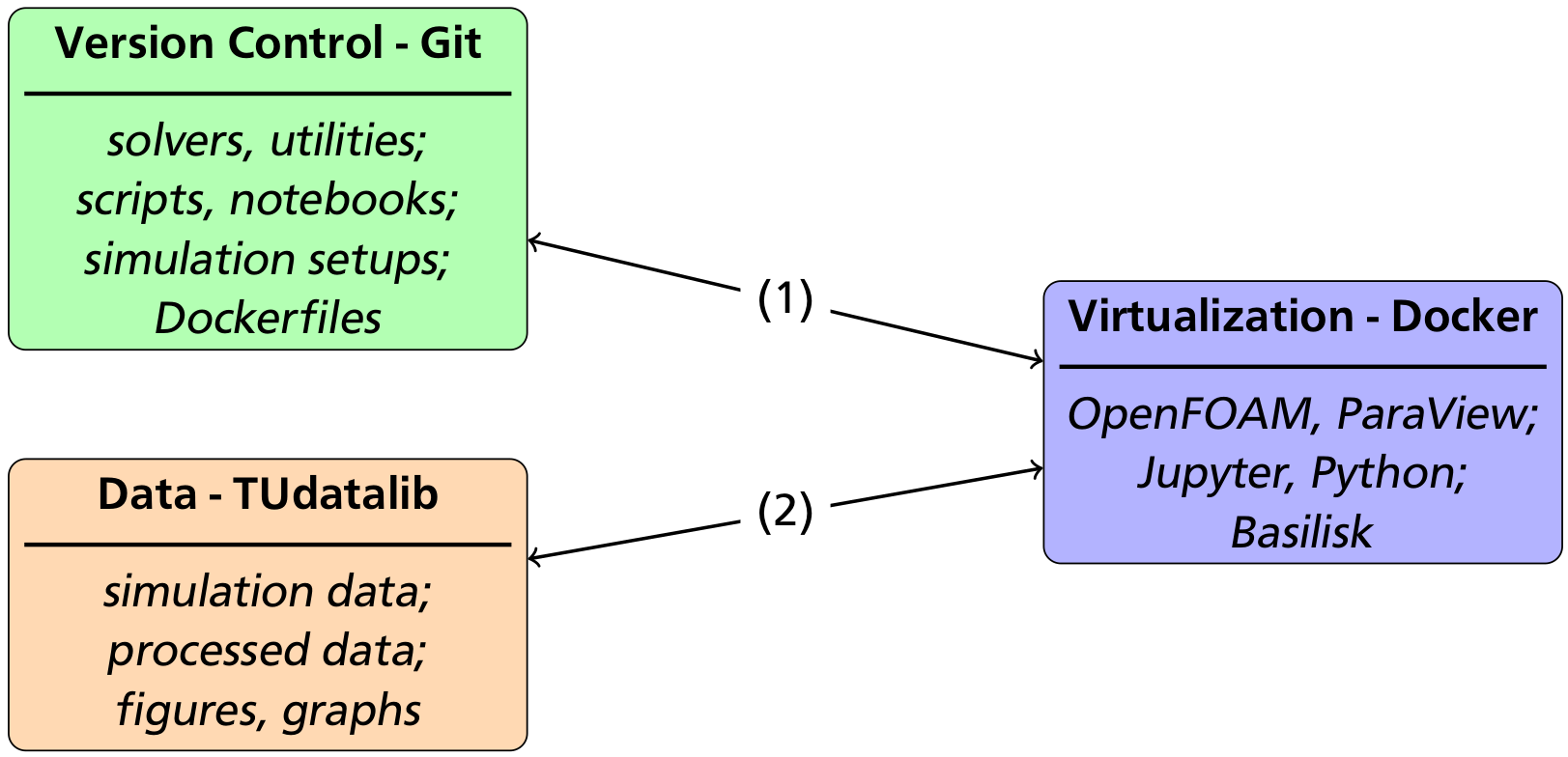
- https://github.com/AndreWeiner/phd_notebooks
- https://github.com/AndreWeiner/phd_basilisk
- https://github.com/AndreWeiner/phd_openfoam
Solution based on Git/Github, Docker/Dockerhub and TUDatalib.
ML Challenges
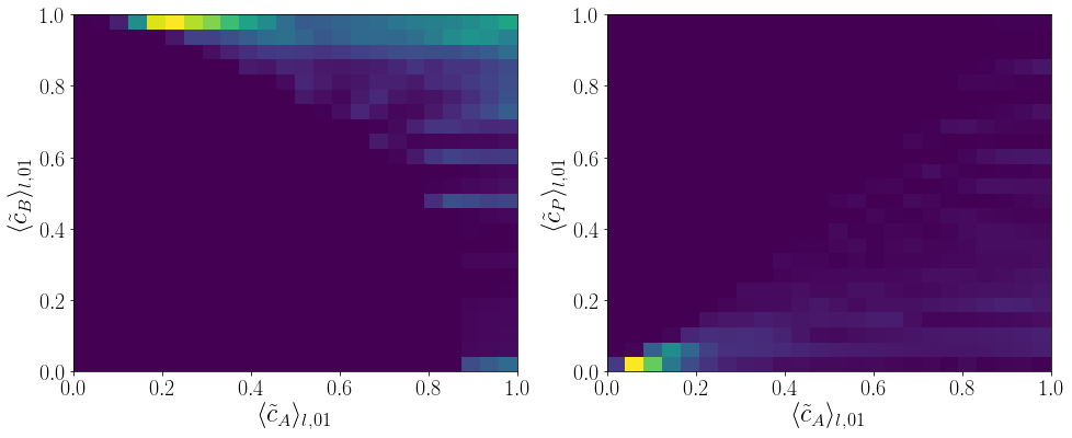
Feature density for the source terms of a parallel-consecutive reaction of type $A+B\rightarrow P$ and $A+P\rightarrow S$.
Video by courtesy of David Merker.
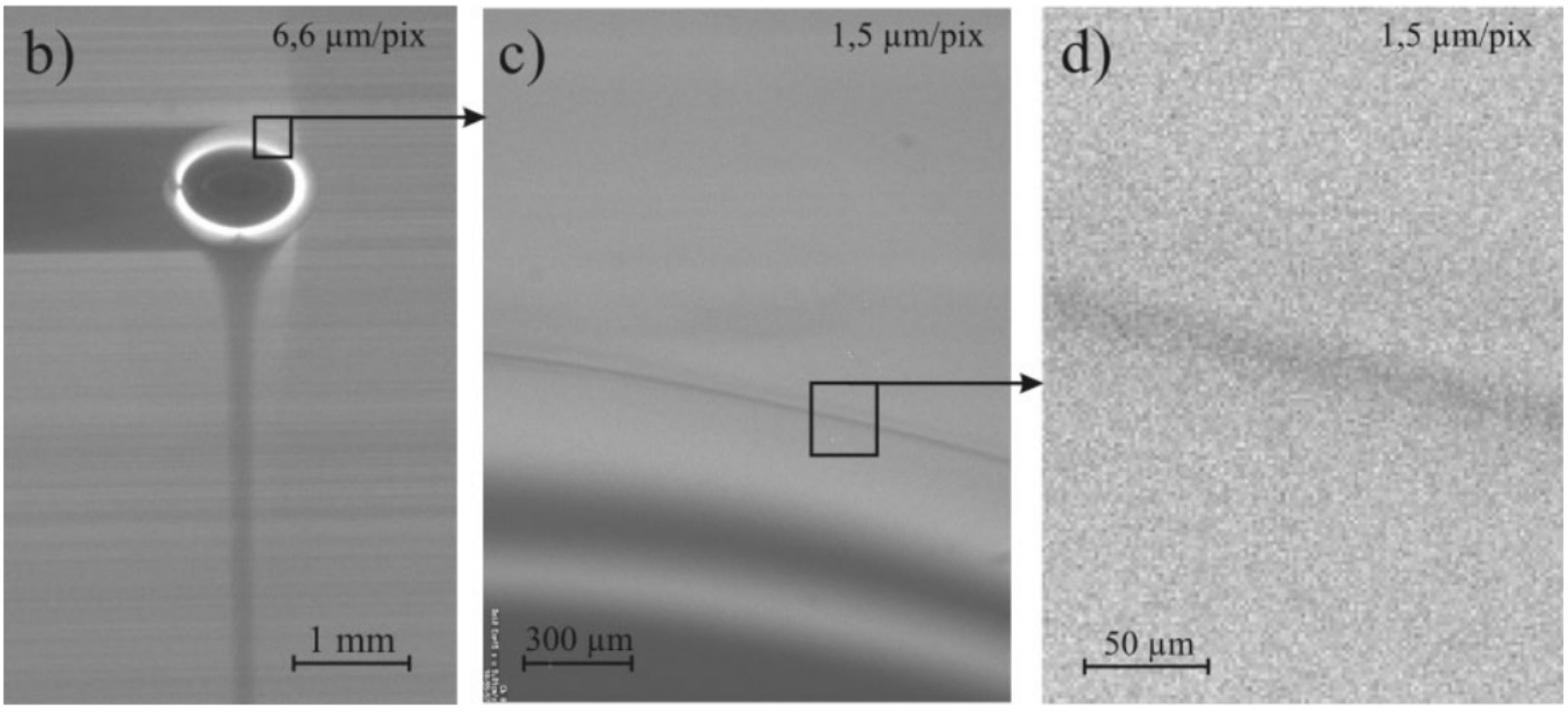
Pendant bubble method
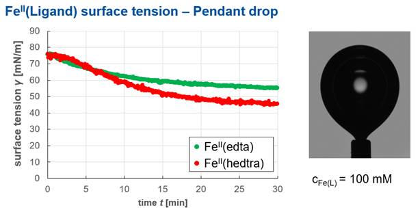
Image by courtesy of David Merker. Measurement apparatus by dataphysics-instruments.
Bulk species - B
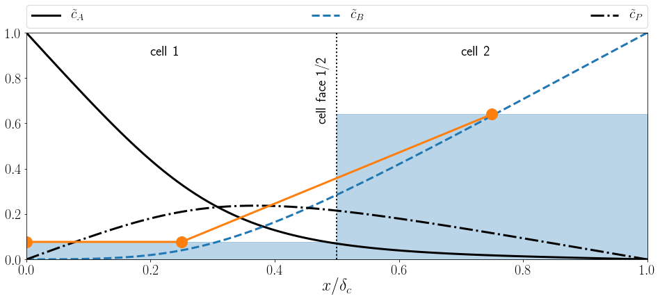 Normalized concentration profile $\tilde{c}_B$ in interface normal direction $x/\delta_c$ for the bulk species (dashed blue line),
average concentration values per cell (shaded blue), and linear reconstruction (orange).
Normalized concentration profile $\tilde{c}_B$ in interface normal direction $x/\delta_c$ for the bulk species (dashed blue line),
average concentration values per cell (shaded blue), and linear reconstruction (orange).
Interpolation error B
Product species - P
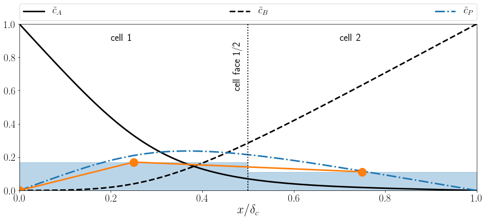 Normalized concentration profile $\tilde{c}_P$ in interface normal direction $x/\delta_c$ for the product species (dash-dotted blue line),
average concentration values per cell (shaded blue), and linear reconstruction (orange).
Normalized concentration profile $\tilde{c}_P$ in interface normal direction $x/\delta_c$ for the product species (dash-dotted blue line),
average concentration values per cell (shaded blue), and linear reconstruction (orange).
Interpolation error P
Source term
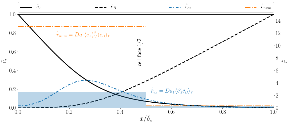 Reaction source profile $\dot{\tilde{r}}$ in interface normal direction $x/\delta_c$ (dash-dotted blue line),
cell average of $\dot{\tilde{r}}$ (shaded blue), and product of averages (orange). The Damköhler number is defined as $Da=kd_b/U_b$.
Reaction source profile $\dot{\tilde{r}}$ in interface normal direction $x/\delta_c$ (dash-dotted blue line),
cell average of $\dot{\tilde{r}}$ (shaded blue), and product of averages (orange). The Damköhler number is defined as $Da=kd_b/U_b$.
Feature selection
Idea: ranking of feature importance.
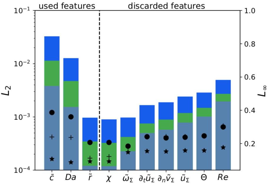
algorithms
- regression forest
- sequential backward selection
- sequential forward selection
example (left)
$f_m = f_m(\bar{c},Da,\tilde{r})$
ML model assessment
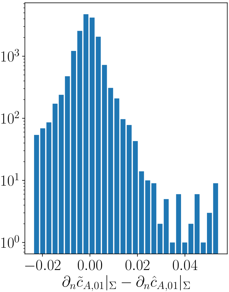
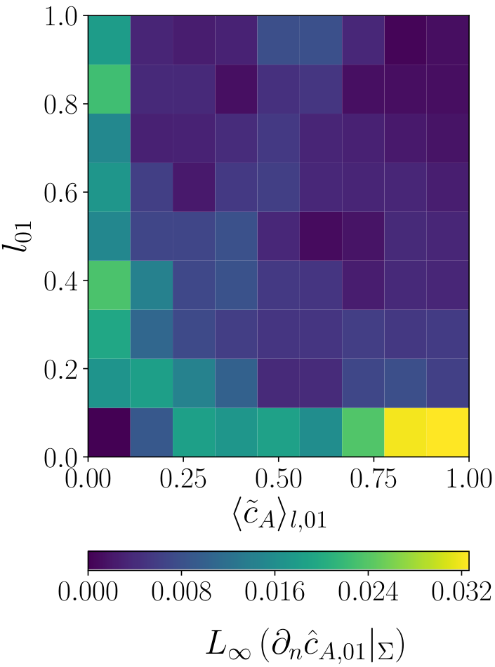
Histogram (left) and heatmap (right) of the label error for the transfer species (A). Reminder: the height of a bar in a histogram depicts the number of instances in the range the bar covers. The index $01$ indicates a min-max-scaling.