Machine Learning in Fluid Dynamics
- an overview -
Andre Weiner, Chair of Fluid Mechanics

| 01 | machine learning tasks regression, classification, clustering, ... |
| 02 | optimizing settings with Bayesian optimization |
| 03 | understanding turbulent flows with modal decomposition |
| 04 | closed-loop flow control with model-based deep reinforcement learning |
machine learning tasks
regression, classification, clustering, ...
think in terms of machine learning tasks
(regression, classification, ...)
rather than specific algorithms
(neural networks, Gaussian processes, ...)
regression: matching inputs and continuous outputs


classification: matching inputs and discrete outputs


dim. reduction: finding low-dim. representations


clustering: grouping similar data points


reinforcement learning: sequential decision making (control) under uncertainty


machine learning algorithms are essential to solve these tasks in higher dimensions
many problems need to be broken up into multiple tasks
reduced-order modeling
-
dimensionality reduction
maps high- to low-dim. inputs/outputs -
regression or classification
low-dimensional input-output mappings -
back-projection (optional)
inverts step 1. for new predictions
outlier detection (extreme events)
-
dimensionality reduction
maps high- to low-dim. representations -
clustering or classification
low similarity or class probabilities
formulating sensible tasks requires
domain knowledge
optimizing settings
with Bayesian optimization
joint work with
- Janis Geise (TU Dresden)
- Tomislav Marić (TU Darmstadt)
- M. Elwardi Fadeli (TU Darmstadt)
- Alessandro Rigazzi (HPE)
- Andrew Shao (HPE)


GAMG - generalized geometric algebraic multigrid
excellent introduction by Fluid Mechanics 101
full GAMG entry in fvSolution
						p
{
	solver                    GAMG;
	smoother                  DICGaussSeidel;
	tolerance                 1e-06;
	relTol                    0.01;
	cacheAgglomeration        yes;
	nCellsInCoarsestLevel     10;
	processorAgglomerator     none;
	nPreSweeps                0;
	preSweepsLevelMultiplier  1;
	maxPreSweeps              10;
	nPostSweeps               2;
	postSweepsLevelMultiplier 1;
	maxPostSweeps             10;
	nFinestSweeps             2;
	interpolateCorrection     no;
	scaleCorrection           yes;
	directSolveCoarsest       no;
	coarsestLevelCorr
	{
		solver          PCG;
		preconditioner  DIC;
		tolerance       1e-06;
		relTol          0.01;
	}
}
optimal settings depend on
- coefficient matrix
- flow physics
- discretization
- parallelization
- hardware
- ...
$\rightarrow$ high-dim. search space with uncertainty

~15% runtime reduction
references & examples (GitHub)
understanding turbulent flows
with modal decomposition
joint work with
- Janis Geise (TU Dresden)
- Sebastian Spinner (DLR)
- Richard Semaan (f. TU Braunschweig)
flow past a cylinder: $|\mathbf{u}|$ at $Re=dU_\mathrm{in}/\nu=100$
data $=$ spatial patterns $\times$ temporal patterns
$|\mathbf{u}|$ at $Re=dU_\mathrm{in}/\nu=3700$; DNS setup based on
O. Lehmkuhl et al. (2013)

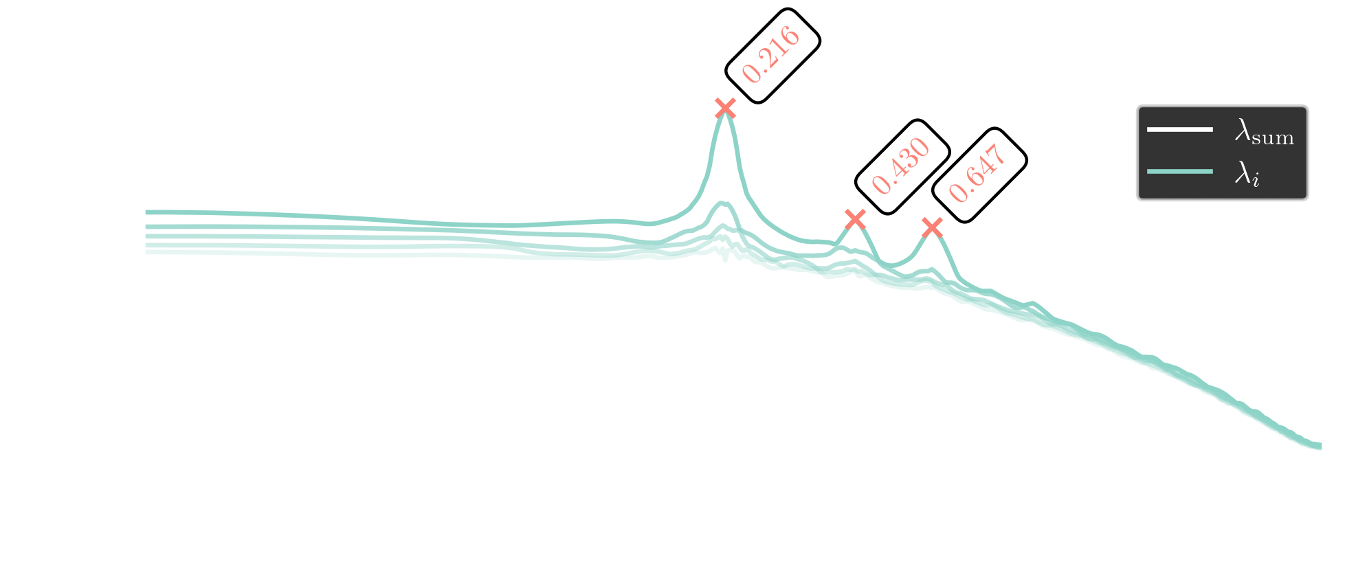
PSD of force coefficients (p-Welch, 4 segments)
$St=fT_\mathrm{conv}$ and $T_\mathrm{conv}=d/U_\mathrm{in}$
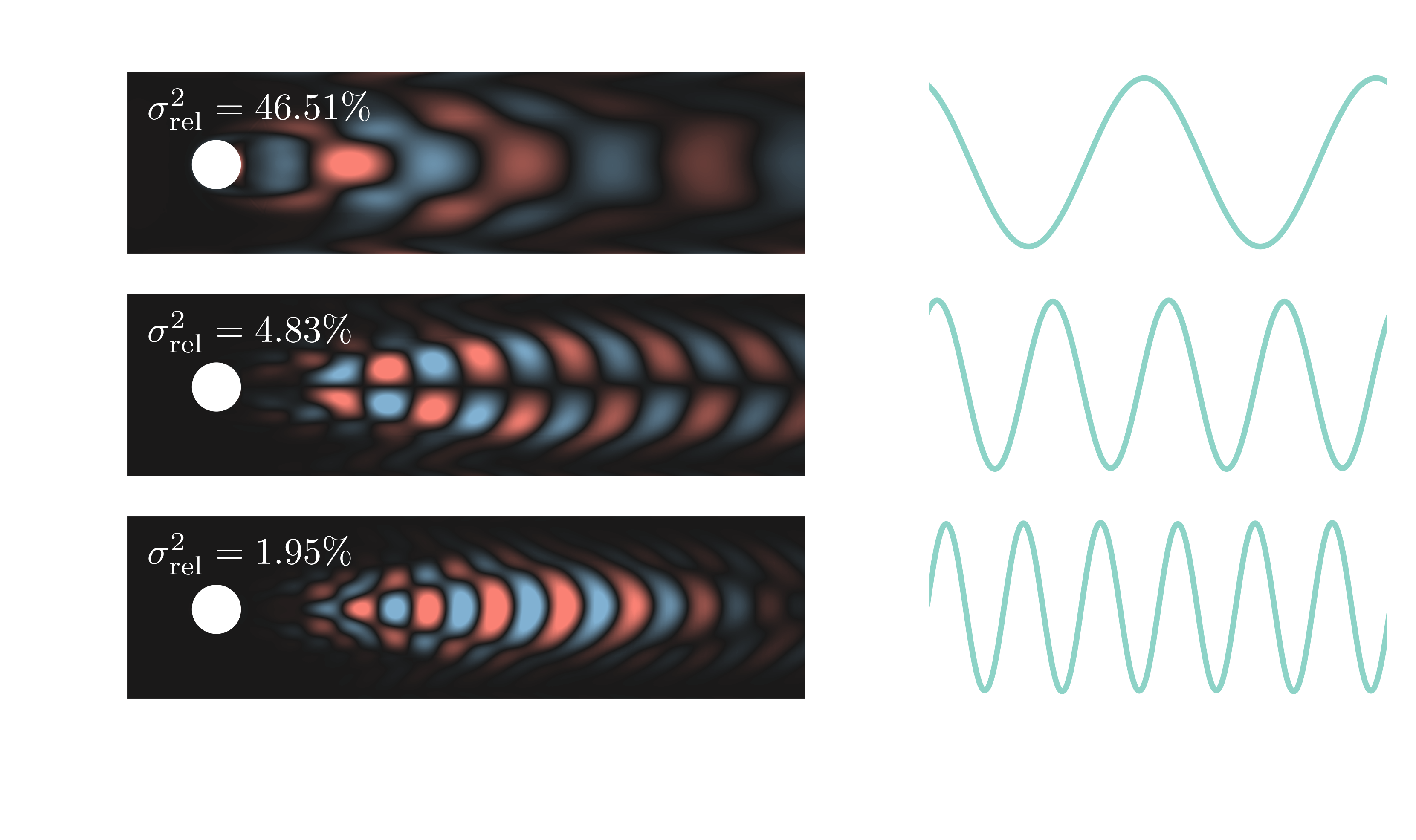
adaptive sin-taper spectral POD
refer to B. C. Y. Yeung, O. T. Schmidt (2024)
vortex shedding mode
$St\approx 0.22$, streamwise component
Airbus XRF-1 shock buffet mode ($Re_\infty = 3.3\times 10^6$, $Ma_\infty =0.84$, $\alpha=-4^\circ$); DDES by S. Spinner (DLR)
references & examples
closed-loop flow control
with model-based deep reinforcement learning
joint work with Janis Geise (TU Dresden)

closed-loop control benchmark, $Re=100$
instantaneous reward $R_n$
$$ R_n = 3 - (c_{x,n} + 0.1 |c_{y,n}|) $$
$c_{i, n}$ - force coefficients at step $n$
evaluation of optimal policy (control law)
evaluation of optimal policy (control law)
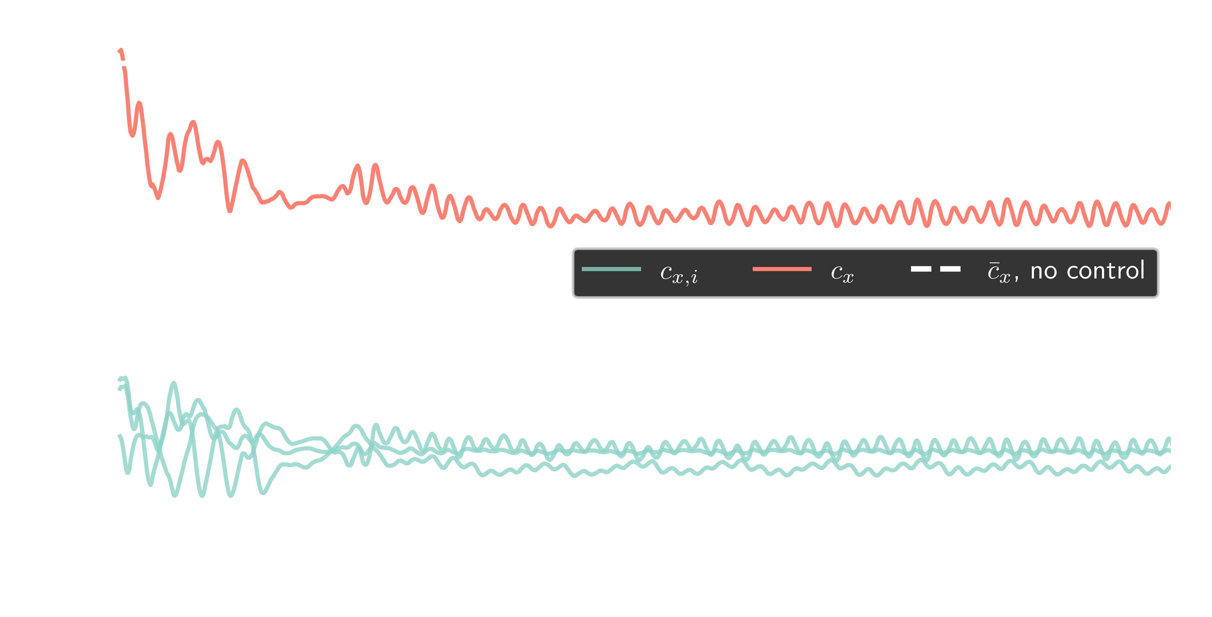
drag reduction by approx. $25\%$
references