Bayesian
parameter & design
optimization

Andre Weiner, Tomislav Marić

01	Gaussian processes (GP) from Gaussians distributions to GPs
03	example 1: GAMG settings optimal solver settings for fast simulations
04	example 2: heat exchanger balancing pressure loss and heat transfer

Gaussian process regression

process with $d$ random variables

$\boldsymbol{X} = \left[X_1, X_2, \ldots, X_d \right]^T$, $\boldsymbol{X} \in \mathbb{R}^{d\times 1}$

expectation (mean value)

$\mu_i = \mathbb{E}\left[X_i\right]$, $\boldsymbol{\mu} = \left[\mu_1, \mu_2, \ldots, \mu_d\right]^T$, $\boldsymbol{\mu} \in \mathbb{R}^{d\times 1}$

covariance

$\sigma_{ij} = \mathbb{E}\left[(X_i-\mu_i)(X_j-\mu_j)\right]$, $\mathbf{\Sigma} \in \mathbb{R}^{d\times d}$

motivation

$\mathbf{y} = \mathbf{x} - \boldsymbol{\mu}$, $\Sigma = \mathbf{Q \Lambda Q}^T$, $\tilde{\mathbf{y}} = \mathbf{Q}^T \mathbf{y}$

normalization in principal coordinates

$\tilde{\mathbf{z}}^T = \tilde{\mathbf{y}}^T \mathbf{\Lambda}^{-1/2}$

back transformation and substitution

$\mathbf{z} = \mathbf{Q}\tilde{\mathbf{z}} = \mathbf{Q}\mathbf{\Lambda}^{-1/2}\mathbf{Q}^T \mathbf{y} = \mathbf{\Sigma}^{-1/2} \mathbf{y} = \mathbf{\Sigma}^{-1/2} (\mathbf{x} - \boldsymbol{\mu})$

Mahalanobis distance

$d_m^2 = |\mathbf{z}|^2 = \mathbf{z}^T\mathbf{z} = (\mathbf{x} - \boldsymbol{\mu})^T\mathbf{\Sigma}^{-1} (\mathbf{x} - \boldsymbol{\mu})$

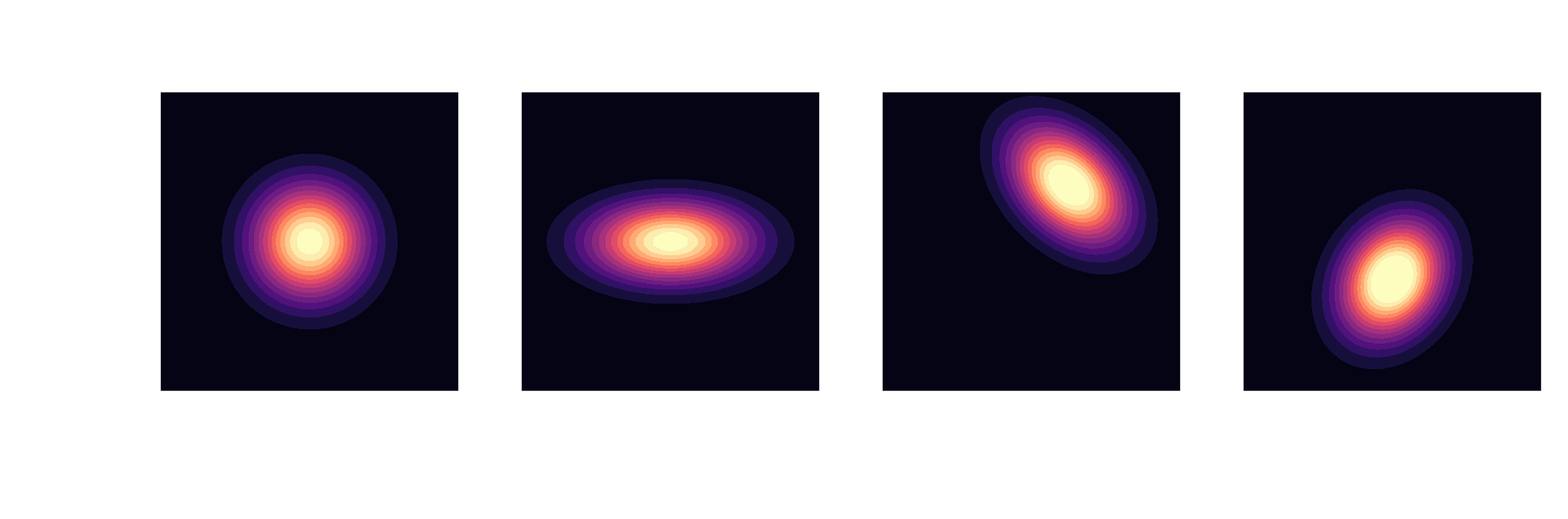
multivariate Gaussian distribution

$$ p(\mathbf{x}) = \frac{1}{\sqrt{(2\pi)^d \mathrm{det}(\mathbf{\Sigma})}}\mathrm{exp}\left( -\frac{1}{2}(\mathbf{x}-\boldsymbol{\mu})^T\mathbf{\Sigma}^{-1}(\mathbf{x}-\boldsymbol{\mu}) \right) $$

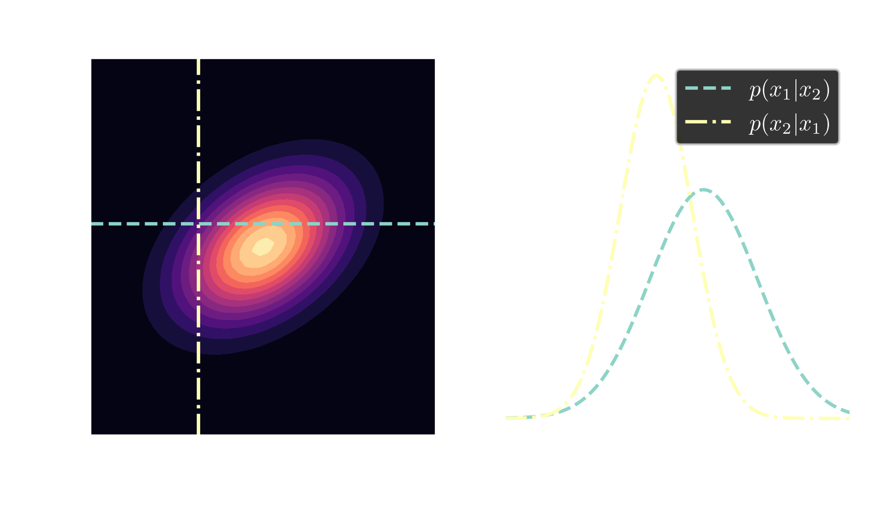
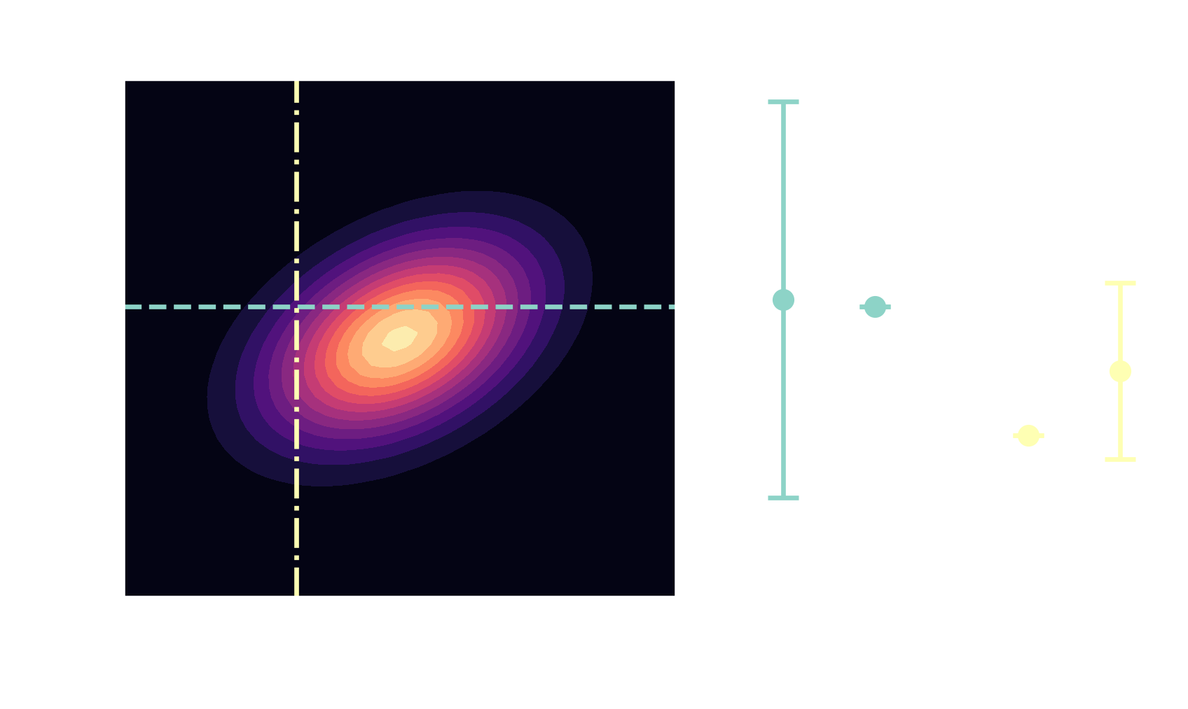
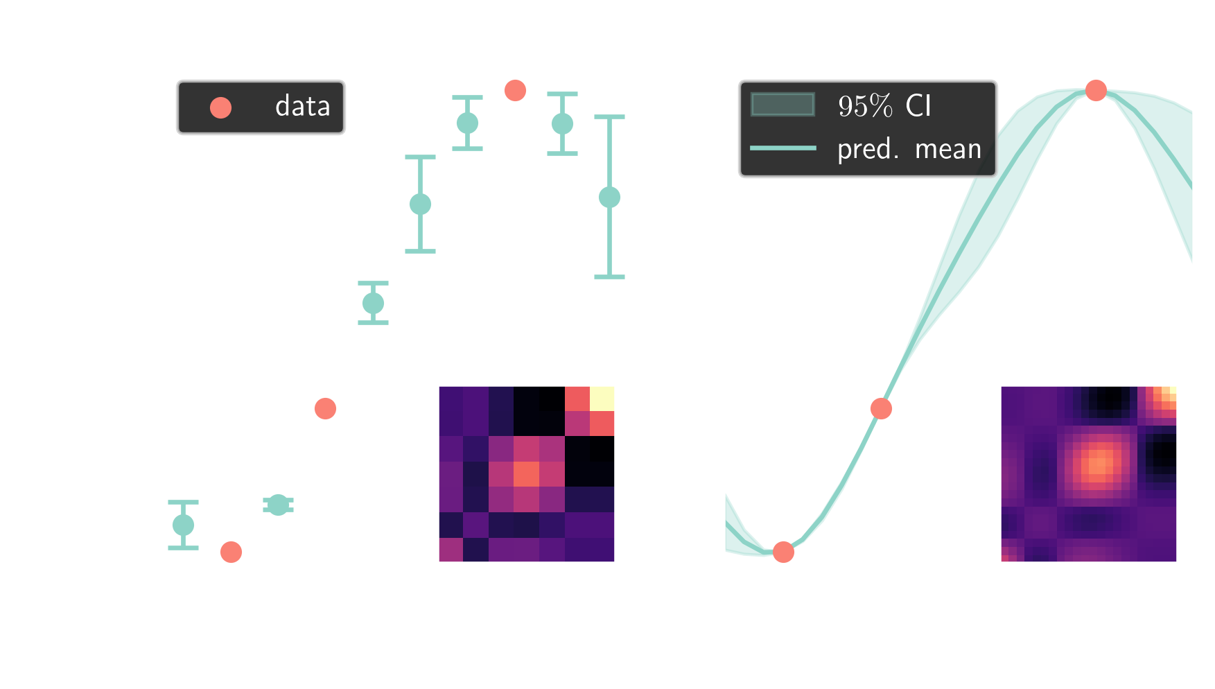
Gaussians are closed under conditioning

$$ \boldsymbol{\mu}=\begin{bmatrix} \boldsymbol{\mu}_A \\ \boldsymbol{\mu}_B \end{bmatrix}, \quad \mathbf{\Sigma} = \begin{bmatrix} \mathbf{\Sigma}_{AA} & \mathbf{\Sigma}_{AB}\\ \mathbf{\Sigma}_{BA} & \mathbf{\Sigma}_{BB} \end{bmatrix} $$

$$ \boldsymbol{\mu}_{A|B}= \boldsymbol{\mu}_A + \mathbf{\Sigma}_{AB}\mathbf{\Sigma}^{-1}_{BB}\left(\mathbf{x}_B-\mathbf{\mu}_B\right) $$ $$ \mathbf{\Sigma}_{A|B} = \mathbf{\Sigma}_{AA} - \mathbf{\Sigma}_{AB} \mathbf{\Sigma}^{-1}_{BB} \mathbf{\Sigma}_{BA} $$ posterior $\quad\mathbf{X}_{A|B} \sim \mathcal{N}(\boldsymbol{\mu}_{A|B}, \mathbf{\Sigma}_{A|B})$

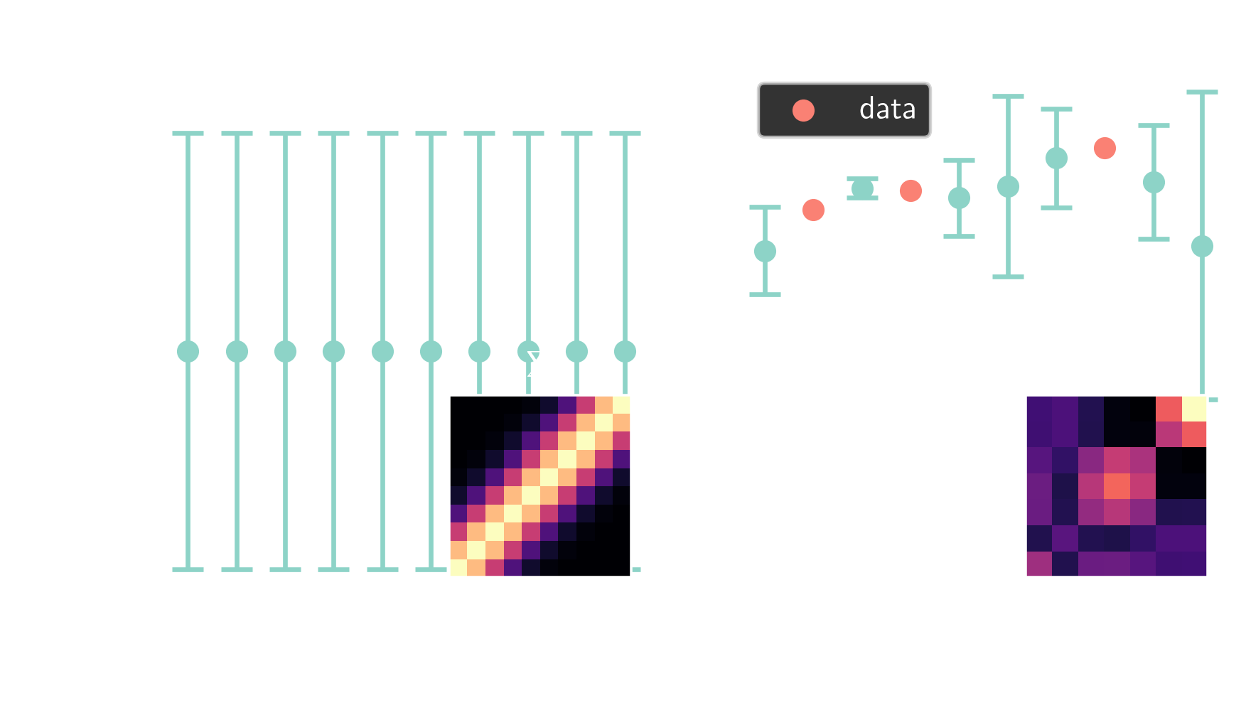
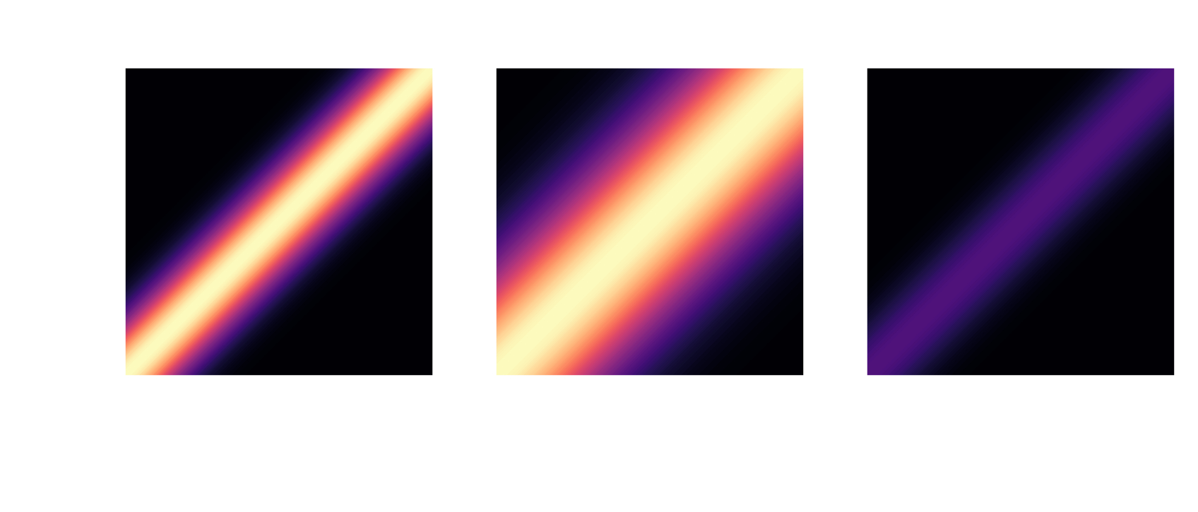
from multivariate Gaussians $$ \boldsymbol{X} \sim \mathcal{N}(\boldsymbol{\mu}, \mathbf{\Sigma}) $$

... to Gaussian processes $$ f(\boldsymbol{x}) \sim \mathcal{GP}(m(\boldsymbol{x}), k(\boldsymbol{x}, \boldsymbol{x}^\prime)) $$

RBF kernel: $ \quad k(x, x^\prime) = \sigma^2 \mathrm{exp}\left(-\frac{|x - x^\prime|^2}{2l^2}\right) $

example 1:

optimizing GAMG settings

joint work with:

Janis Geise (TU Dresden)
Tanuj Ravi (TU Dresden)
Tomislav Marić (TU Darmstadt)
M. Elwardi Fadeli (TU Darmstadt)
Alessandro Rigazzi (HPE)
Andrew Shao (HPE)

code: github.com/JanisGeise/BayesOpt_solverSettings

GAMG - generalized geometric algebraic multigrid

excellent introduction by Fluid Mechanics 101

full GAMG entry in fvSolution

						p
{
	solver                    GAMG;
	smoother                  DICGaussSeidel;
	tolerance                 1e-06;
	relTol                    0.01;
	cacheAgglomeration        yes;
	nCellsInCoarsestLevel     10;
	processorAgglomerator     none;
	nPreSweeps                0;
	preSweepsLevelMultiplier  1;
	maxPreSweeps              10;
	nPostSweeps               2;
	postSweepsLevelMultiplier 1;
	maxPostSweeps             10;
	nFinestSweeps             2;
	interpolateCorrection     no;
	scaleCorrection           yes;
	directSolveCoarsest       no;
	coarsestLevelCorr
	{
		solver          PCG;
		preconditioner  DIC;
		tolerance       1e-06;
		relTol          0.01;
	}
}

optimal settings depend on

coefficient matrix
- flow physics
- discretization

parallelization
hardware
...

$\rightarrow$ high-dim. search space with uncertainty

reduce runtime without sacrificing accuracy

						PIMPLE
{
    ...

    residualControl
    {
        "(U|p)"
        {
            relTol          0;
            tolerance       1e-05;
        }
    }
}

elapsed time for 50 steps; 2D cylinder flow

implementation outline

Ax for BayesOpt
SmartSim for orchestration
~100 lines Python script

						ens = exp.create_ensemble(
    name=f"int_{time_idx}_trial_{'_'.join(keys_str)}",
    params=params,
    perm_strategy="step",
    run_settings=rs,
    batch_settings=bs
)
base_case_path = config["simulation"]["base_case"]
ens.attach_generator_files(to_configure=base_case_path)
exp.generate(ens, overwrite=True, tag="!")
exp.start(ens, block=True, summary=True)

search space definition in config.yaml

						smoother:
	name: "smoother"
	type: "choice"
	value_type: "str"
	is_ordered: False
	sort_values: False
	values: ["FDIC", "DIC", "DICGaussSeidel", "symGaussSeidel", "nonBlockingGaussSeidel", "GaussSeidel"]
nFinestSweeps:
	name: "nFinestSweeps"
	type: "range"
	value_type: "int"
	bounds: [1, 10]
...

~10-15% runtime reduction

$\rightarrow$ example 2

THE END

Thank you for you attention!

data-driven modeling SIG

github.com/OFDataCommittee/openfoam-smartsim