Data-driven modeling, optimization, and control in CFD
Andre Weiner, Chair of Fluid Mechanics

| 01 | machine learning tasks regression, classification, clustering, ... |
| 02 | optimizing GAMG settings with Bayesian optimization |
| 03 | modeling a turbulent flow with dynamic mode decomposition |
| 04 | closed-loop flow control with model-based deep reinforcement learning |
machine learning tasks
regression, classification, clustering, ...
Think in terms of machine learning tasks (regression, classification, ...) rather than specific algorithms (neural networks, Gaussian processes, ...).
regression: matching inputs and continuous outputs


classification: matching inputs and discrete outputs


dim. reduction: finding low-dim. representations


clustering: grouping similar data points


reinforcement learning: sequential decision making (control) under uncertainty


optimizing GAMG settings
with Bayesian optimization (BayesOpt)
joint work with:
- Janis Geise (TU Dresden)
- Tomislav Marić (TU Darmstadt)
- M. Elwardi Fadeli (TU Darmstadt)
- Alessandro Rigazzi (HPE)
- Andrew Shao (HPE)
references:
GAMG - generalized geometric algebraic multigrid
excellent introduction by Fluid Mechanics 101
full GAMG entry in fvSolution
						p
{
	solver                    GAMG;
	smoother                  DICGaussSeidel;
	tolerance                 1e-06;
	relTol                    0.01;
	cacheAgglomeration        yes;
	nCellsInCoarsestLevel     10;
	processorAgglomerator     none;
	nPreSweeps                0;
	preSweepsLevelMultiplier  1;
	maxPreSweeps              10;
	nPostSweeps               2;
	postSweepsLevelMultiplier 1;
	maxPostSweeps             10;
	nFinestSweeps             2;
	interpolateCorrection     no;
	scaleCorrection           yes;
	directSolveCoarsest       no;
	coarsestLevelCorr
	{
		solver          PCG;
		preconditioner  DIC;
		tolerance       1e-06;
		relTol          0.01;
	}
}
optimal settings depend on
- coefficient matrix
- flow physics
- discretization
- parallelization
- hardware
- ...
$\rightarrow$ high-dim. search space with uncertainty
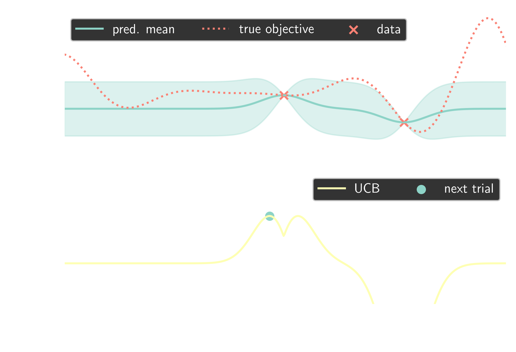
Bayesian optimization
optimization of black-box objective function guided by probabilistic surrogate model (Gaussian process)
idea
use BayesOpt to find optimal GAMG settings
for class of simulations

elapsed time for 50 steps; 2D cylinder flow
implementation outline
search space definition in config.yaml
						smoother:
	name: "smoother"
	type: "choice"
	value_type: "str"
	is_ordered: False
	sort_values: False
	values: ["FDIC", "DIC", "DICGaussSeidel", "symGaussSeidel", "nonBlockingGaussSeidel", "GaussSeidel"]
nFinestSweeps:
	name: "nFinestSweeps"
	type: "range"
	value_type: "int"
	bounds: [1, 10]
...

~15% runtime reduction
modeling a turbulent flow
with dynamic mode decomposition (DMD)
joint work with:
- Janis Geise (TU Dresden)
- Richard Semaan (f. TU Braunschweig)
references:
DMD = dimensionality reduction + (linear) regression
advantages
- efficient
- interpretable
- predictive (ROM)
- many extensions
disadvantages
- sensitivity
- white noise
- nonlinearity
- poor predictions
some notation
| nr. state variables | $M$ |
| state vector | $\mathbf{x}_n \in \mathbb{R}^M$ |
| nr. snapshots | $N$ |
| data matrix | $\mathbf{M} = \left[\mathbf{x}_1, \ldots, \mathbf{x}_N \right]^T$ |
dimensionality reduction via SVD
$$\mathbf{M} \approx \mathbf{U}_r\mathbf{\Sigma}_r\mathbf{V}_r^T$$
reduced data matrix
$$\tilde{\mathbf{M}} = \mathbf{U}_r^T\mathbf{M} = \mathbf{\Sigma}_r\mathbf{V}_r^T,\quad \tilde{\mathbf{M}} \in \mathbb{R}^{r\times N}$$
$$N \ll M,\quad r\ll N$$
classical DMD
$$\tilde{\mathbf{x}}_{n+1} = \tilde{\mathbf{A}} \tilde{\mathbf{x}}_{n}$$
$$\underset{\tilde{\mathbf{A}}}{\mathrm{argmin}}\left|\left| \tilde{\mathbf{Y}}-\tilde{\mathbf{A}}\tilde{\mathbf{X}} \right|\right|_2 =\tilde{\mathbf{Y}}\tilde{\mathbf{X}}^\dagger$$
$$\tilde{\mathbf{X}} = \left[\mathbf{x}_1, \ldots, \mathbf{x}_{N-1} \right]^T,\quad \tilde{\mathbf{Y}} = \left[\mathbf{x}_2, \ldots, \mathbf{x}_{N} \right]^T$$

noise-corrupted reduced state vector

noise leads to decaying dynamics
forward-backward-consistent DMD
if $\ \tilde{\mathbf{x}}_{n+1} = \tilde{\mathbf{A}} \tilde{\mathbf{x}}_{n}\ $ then $\ \tilde{\mathbf{A}}^{-1}\tilde{\mathbf{x}}_{n+1} = \tilde{\mathbf{x}}_{n}$
$$\underset{\tilde{\mathbf{A}}}{\mathrm{argmin}}\left|\left| \tilde{\mathbf{Y}}-\tilde{\mathbf{A}}\tilde{\mathbf{X}} \right|\right|_F + \left|\left| \tilde{\mathbf{X}}-\tilde{\mathbf{A}}^{-1}\tilde{\mathbf{Y}} \right|\right|_F$$
reference: O. Azencot et al. (2019)

improved robustness, small frequency error
error propagation - "optimized" DMD
$\tilde{\mathbf{x}}_n \approx \tilde{\mathbf{\Phi}}\tilde{\mathbf{\Lambda}}^{n-1}\tilde{\mathbf{b}}$, $\ \tilde{\mathbf{A}}=\tilde{\mathbf{\Phi}}\tilde{\mathbf{\Lambda}}\tilde{\mathbf{\Phi}}^{-1}$, $\ \tilde{\mathbf{b}} = \tilde{\mathbf{\Phi}}^{-1}\tilde{\mathbf{x}}_1$
$$\underset{\tilde{\mathbf{\lambda}},\tilde{\mathbf{\Phi}}_\mathbf{b}}{\mathrm{argmin}}\left|\left| \tilde{\mathbf{M}}-\tilde{\mathbf{\Phi}}_\mathbf{b}\tilde{\mathbf{V}}_{\mathbf{\lambda}} \right|\right|_F$$
reference: T. Askham, J. N. Kutz (2018)

improved robustness, optimization challenging
multiple constraints and noise identification
$ \tilde{\mathbf{x}}_n = \hat{\mathbf{x}}_n + \tilde{\mathbf{n}}_n $
$\hat{\bar{\mathbf{x}}}_{n+h} = \tilde{\mathbf{\Phi}}\tilde{\mathbf{\Lambda}}^{n+h-1}\tilde{\mathbf{\Phi}}^{-1} \hat{\mathbf{x}}_n$
$L_f = \sum\limits_{n=1}^{N-H}\sum\limits_{h=1}^{H} \left|\tilde{\mathbf{x}}_{n+h} - \hat{\bar{\mathbf{x}}}_{n+h}\right|$
$L_b = \sum\limits_{n=H+1}^{N}\sum\limits_{h=1}^{H} \left|\tilde{\mathbf{x}}_{n-h} - \hat{\bar{\mathbf{x}}}_{n-h}\right|$
final optimization problem
$\underset{\tilde{\mathbf{\lambda}},\tilde{\mathbf{\Phi}}, \tilde{\mathbf{N}}}{\mathrm{argmin}} \left(L_f + L_b\right)$
optimization via
automatic differentiation + gradient descent

early stopping prevents overadjustment to data

prediction error for increasing noise level
$|\mathbf{u}^\prime|$ at $Re=dU_\mathrm{in}/\nu=3700$; DNS setup based on
O. Lehmkuhl et al. (2013)

PSD of force coefficients (p-Welch, 4 segments)
$St=fT_\mathrm{conv}$ and $T_\mathrm{conv}=d/U_\mathrm{in}$

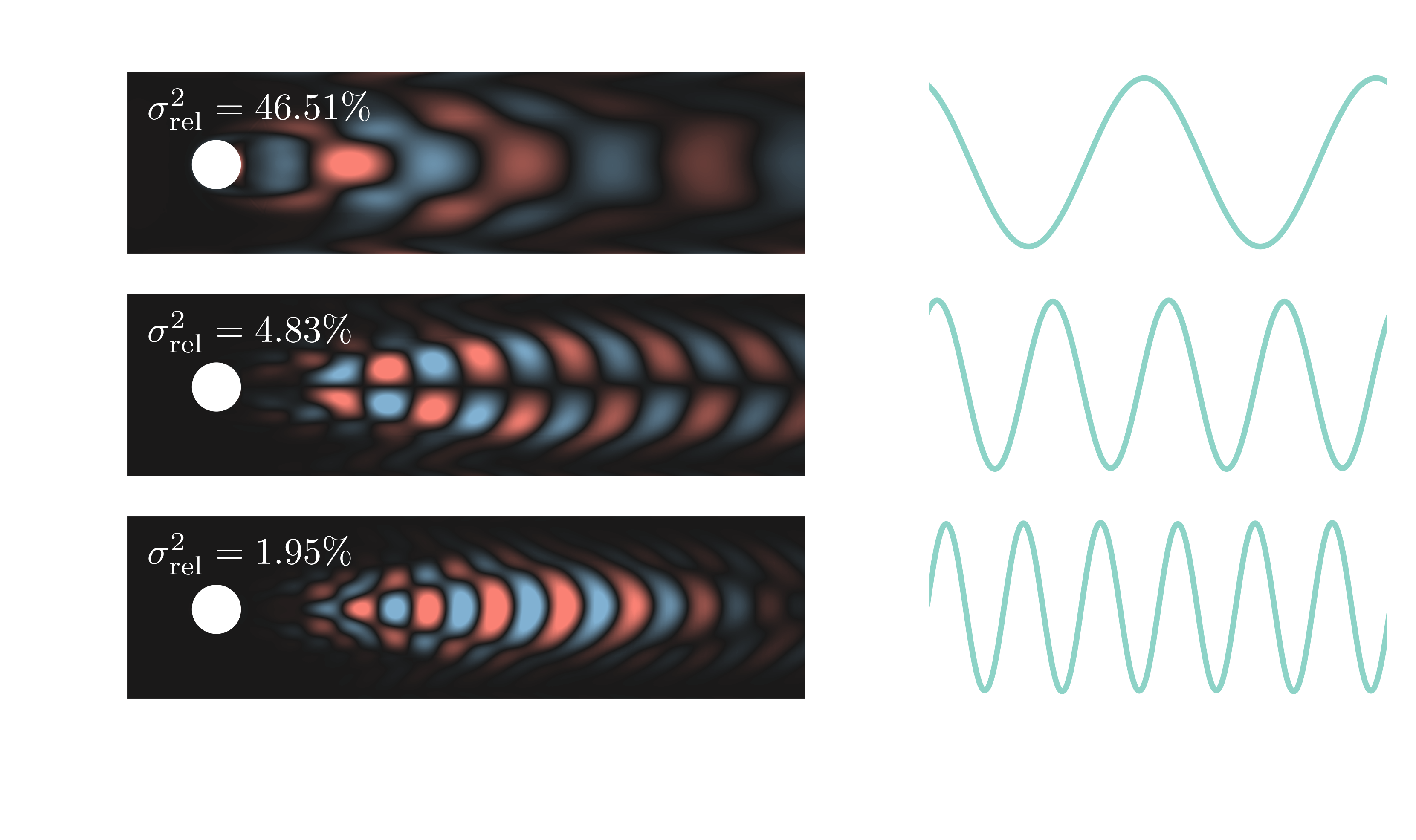
relative and cumulative explained variance
SVD reconstruction with $r=10$
SVD reconstruction with $r=30$
SVD reconstruction with $r=100$
SVD reconstruction with $r=1000$
$|\mathbf{u}^\prime|$ prediction; $r=10$, $H=5f_\mathrm{vs}$
$|\mathbf{u}^\prime|$ vortex shedding mode
closed-loop flow control
with model-based deep reinforcement learning
joint work with Janis Geise (TU Dresden)
references:

closed-loop control benchmark, $Re=100$
evaluation of optimal policy (control law)
separation control, B. Font et al. (2025)
- LES, higher-order spectral elements
- 8 simulations in parallel
- 96 episodes (iterations)
- 6 days turnaround time
- 1152 GPUh (A100)
- $4$ EUR/GPUh $\rightarrow 5$ kEUR
Training cost DrivAer model
- $5$ hours/simulation (1000 MPI ranks)
- $10$ parallel simulations
- $100$ iterations $\rightarrow 20$ days turnaround time
- $20\times 24\times 10\times 1000 \approx 5\times 10^6 $ CPUh
- $0.01-0.05$ EUR/CPUh $\rightarrow 0.5-2$ mEUR
CFD simulations are expensive!
Idea: replace CFD with model(s) in some episodes
Challenge: dealing with surrogate model errors
for e in episodes:
	if not models_reliable():
		sample_trajectories_from_simulation()
		update_models()
	else:
		sample_trajectories_from_models()
	update_policy()
Based on Model Ensemble TRPO.
auto-regressive surrogate models with weights $\theta_m$
$$ m_{\theta_m} : (\underbrace{S_{n-d}, \ldots, S_{n-1}, S_n}_{\hat{S}_n}, A_n) \rightarrow (S_{n+1}, R_{n+1}) $$
$\mathbf{x}_n = [\hat{S}_n, A_n]$ and $\mathbf{y}_n = [S_{n+1}, R_{n+1}]$
$$ L_m = \frac{1}{|D|}\sum\limits_{i}^{|D|} (\mathbf{y}_i - m_{\theta_m}(\mathbf{x}_i))^2 $$
When are the models reliable?
- evaluate policy for every model
- compare to previous policy loss
- switch if loss did not decrease for
at least $N_\mathrm{thr}$ of the models

normalized training time for MEPPO variants
final remarks
data-driven methods in CFD can
- reduce development cost
- improve application design