Data-driven modeling and validation of reactive mass transfer at rising bubbles
Andre Weiner,
TU Braunschweig, Institute of Fluid
Mechanics

These slides and most of the linked resources are licensed under a
Creative Commons Attribution 4.0 International License.
Outline
- Data-driven modeling overview
- Modeling of reactive mass transfer
- Outlook
- Extracting coherent flow structures
- Closure modeling as a control problem
Combining ML and CFD
why and how
Why combine CFD and ML?
CFD
- produces large amounts of complex data
- requires data or representations thereof
ML
- finds patterns in data
- creates useful representations of data
What is data?

primary data: scalar/vector fields, boundary fields, integral values
# log.rhoPimpleFoam Courant Number mean: 0.020065182 max: 0.77497916 deltaT = 6.4813615e-07 Time = 1.22219e-06 PIMPLE: iteration 1 diagonal: Solving for rho, Initial residual = 0, Final residual = 0, No Iterations 0 DILUPBiCGStab: Solving for Ux, Initial residual = 0.0034181127, Final residual = 6.0056507e-05, No Iterations 1 DILUPBiCGStab: Solving for Uy, Initial residual = 0.0052004883, Final residual = 0.00012352706, No Iterations 1 DILUPBiCGStab: Solving for e, Initial residual = 0.06200185, Final residual = 0.0014223046, No Iterations 1 limitTemperature limitT Lower limited 0 (0%) of cells limitTemperature limitT Upper limited 0 (0%) of cells limitTemperature limitT Unlimited Tmax 329.54945 Unlimited Tmin 280.90821Checking geometry... ... Mesh has 2 solution (non-empty) directions (1 1 0) All edges aligned with or perpendicular to non-empty directions. Boundary openness (1.4469362e-19 3.3639901e-21 -2.058499e-13) OK. Max cell openness = 2.4668495e-16 OK. Max aspect ratio = 3.0216602 OK. Minimum face area = 7.0705331e-08. Maximum face area = 0.00033983685. Face area magnitudes OK. Min volume = 1.2975842e-10. Max volume = 6.2366859e-07. Total volume = 0.0017254212. Cell volumes OK. Mesh non-orthogonality Max: 60.489216 average: 4.0292071 Non-orthogonality check OK. Face pyramids OK. Max skewness = 1.1453509 OK. Coupled point location match (average 0) OK.
secondary data: log files, input dictionaries, mesh quality metrics, ...
Examples for data-driven workflows

Example: creating a surrogate or reduced-order model based on numerical data.

Example: creating a space and time dependent boundary condition based on numerical or experimental data.

Example: creating closure models based on numerical data.

Example: active flow control or shape optimization.
But how exactly does it work?
ML is not a generic problem solver ...
Supervised learning

Creating a mapping from features to labels based on examples.
Unsupervised learning


Finding patterns in unlabeled data.
(Deep) Reinforcement learning

Create an intelligent agent that learns to map states to actions such that cumulative rewards are maximized.
What if my problem does not fit into these categories?
$\rightarrow$ mathematical, physical, numerical modeling
Reactive mass transfer at rising bubbles
A single-phase simulation approach to compute the mass transfer at rising bubbles
https://github.com/AndreWeiner/sgs_model_test_transient
Joint work with D. Bothe, CMY. Claassen, IR. Hierck, JAM. Kuipers, MW. Baltussen.
Gas-liquid reactors
micro reactor
size: millimeter
source: SPP 1740
prediction of
- mass transfer
- enhancement
- mixing
- conversion
- selectivity
- yield
- ...
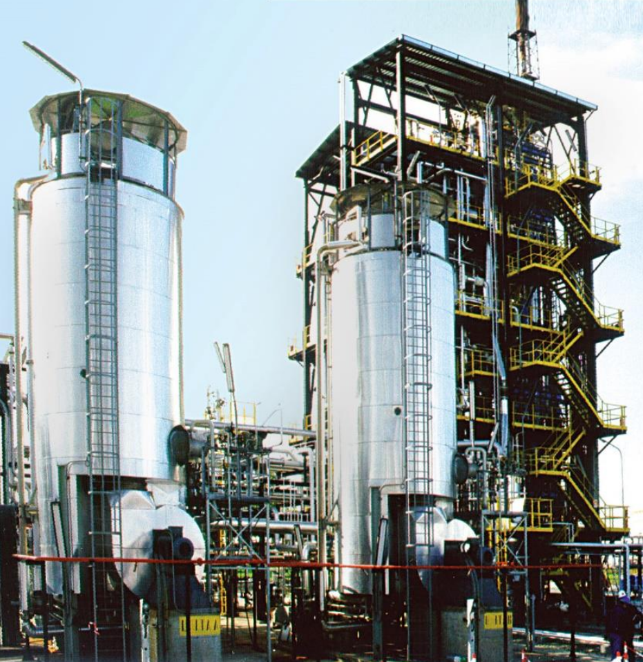
bubble column reactor
size: meter
source: R. M. Raimundo, ENI
Specimen calculation
$d_b=1~mm$ water/oxygen at room temperature
- $Pe = Sc\ Re = \nu_l / D_{O_2} \cdot U_b d_b/\nu_l \approx 10^5 $
- $$ Re\approx 250;\quad \delta_h/d_b \propto Re^{-1/2};\quad\delta_h\approx 45~\mu m $$
- $$ Sc\approx 500;\quad \delta_c/\delta_h \propto Sc^{-1/2};\quad\delta_c\approx 2.5~\mu m $$
$\delta_h/\delta_c$ typically 10 ... 100
feasible simulations up to $Pe\approx 10000$ (3D, HPC)
Why we might be interested in a simplified simulation approach:
- perform parameter studies
- validate boundary layer models
- generate data for ML-based models
- ...
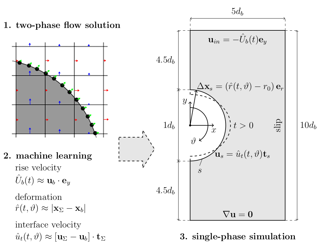
Idea: decoupling of two-phase flow and species transport
1. Two-phase flow simulation (Volume-of-Fluid)
2. Parametrization of shape and interfacial velocity
3. Geometry generation and export (STL format)
4. Single phase mesh
5. Flow solution
6. Species transport
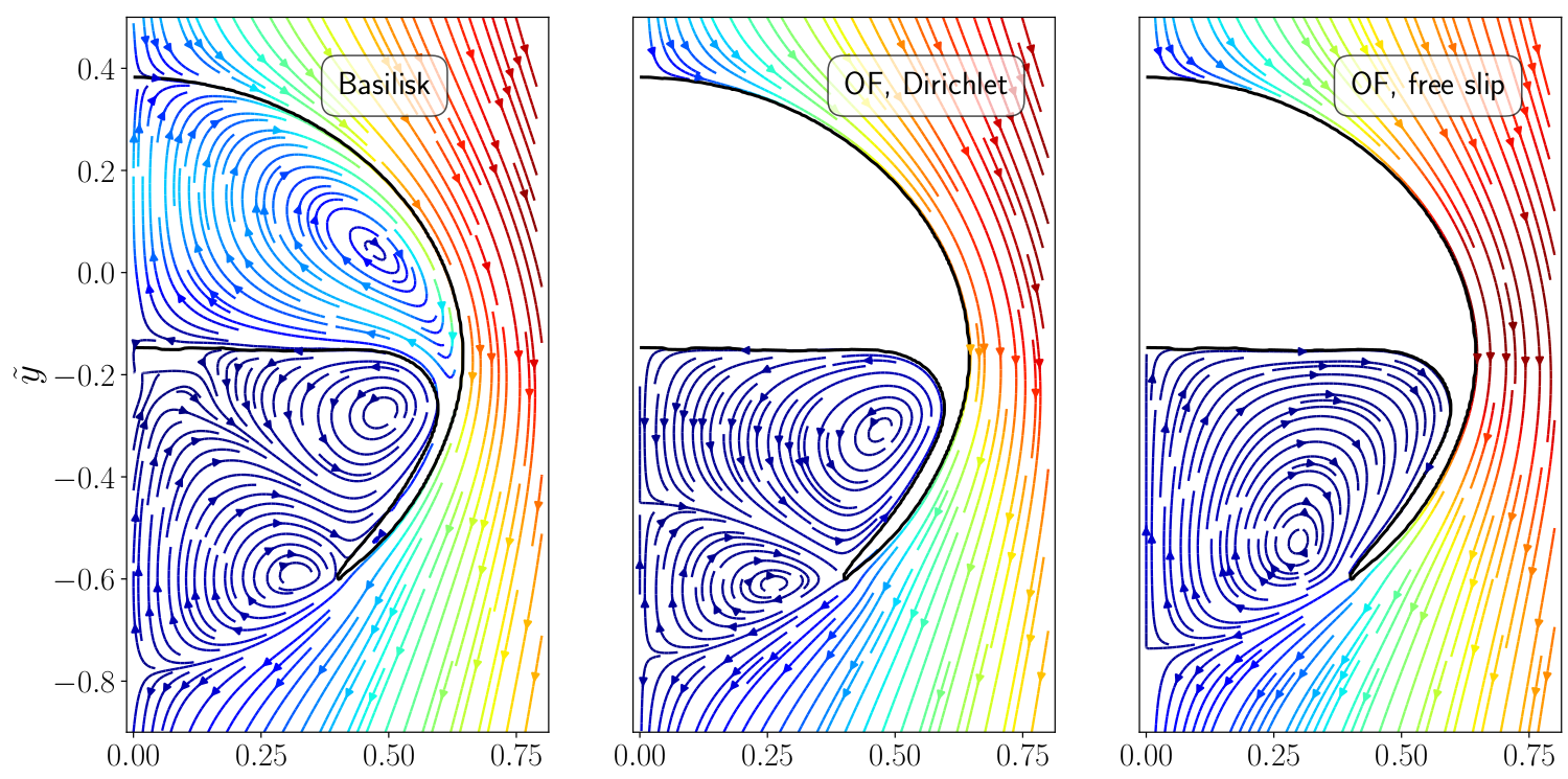
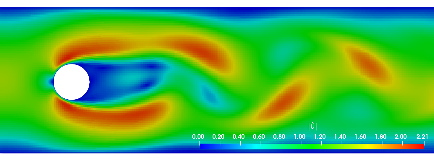
Comparison of two-phase and single-phase flow fields.
Influence of bubble size on local selectivity.
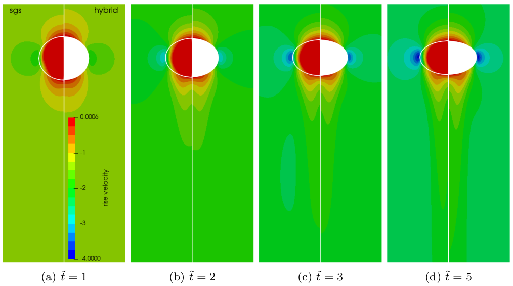
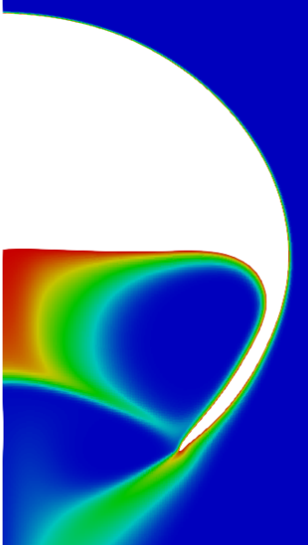
Two-phase velocity field (left half) versus single-phase velocity field (right half); speed-up of 20-40x with 120x finer mesh at surface.
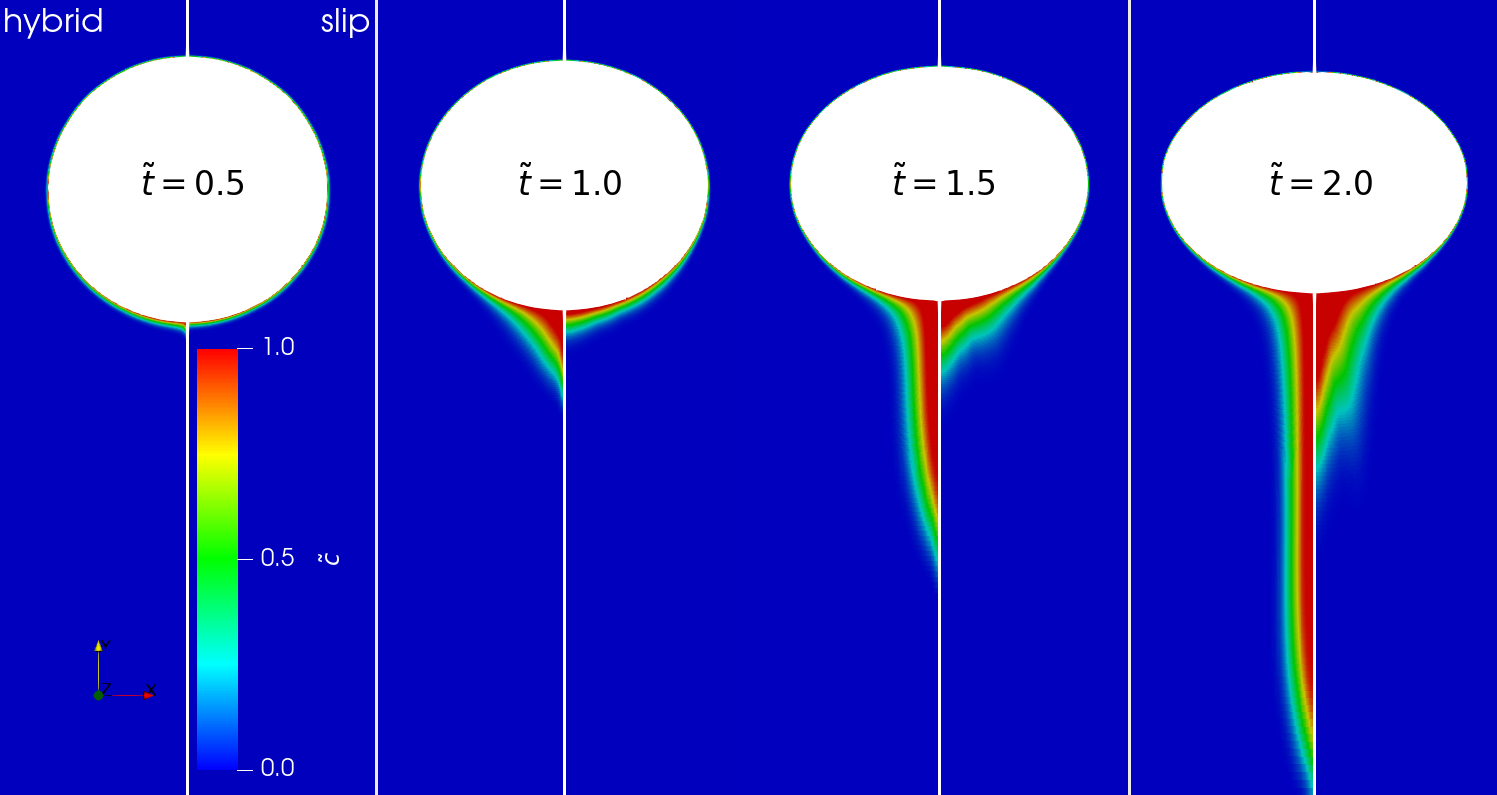
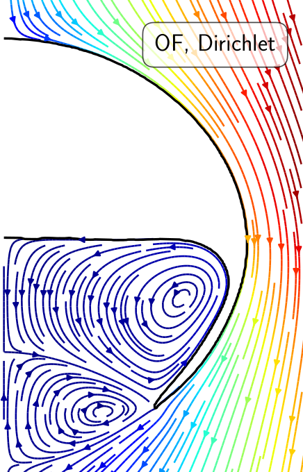
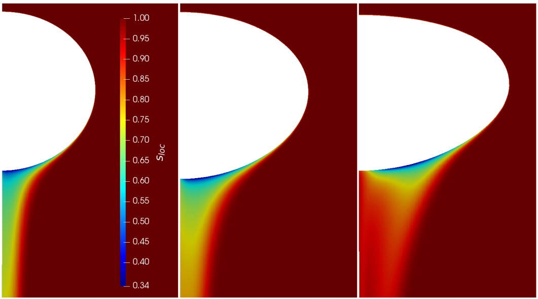
Comparison of concentration fields: data-driven vs. free-slip.
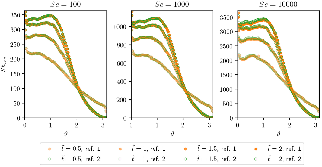
Local Sherwood number for selected time instances.
Inlet boundary condition - first model:
$$ \mathbf{u}_{in} = -\tilde{U}_b\mathbf{e}_y $$
$\tilde{U}_b$ - the bubble's terminal velocity
What would be a more suitable Ansatz for $\tilde{U}_b$?
- $\tilde{U}_b = f_\theta(\tilde{t})$
- $\tilde{U}_b = f_\theta(\tilde{t})\tilde{t}$
$\tilde{t}$ - dimensionless time; $f_\theta(\tilde{t})$ - neural network model.
Interface velocity boundary condition - second model:
$$ \mathbf{u}_s = \tilde{u}_t\mathbf{t} $$
$$ \tilde{u}_t = \tilde{u}_t(\vartheta, \tilde{t}) $$
$\tilde{u}_t$ - tangential component of interface velocity vector.

Sine and cosine functions with vertical lines at $0$ and $\pi$.
How can we enforce the correct symmetry in the model?
- $\tilde{u}_t = f_\theta (\vartheta, \tilde{t})\mathrm{sin}(\vartheta)$
- $\tilde{u}_t = f_\theta (\vartheta, \tilde{t})\mathrm{cos}(\vartheta)$
- $\tilde{u}_t = f_\theta (\mathrm{sin}(\vartheta), \tilde{t})\mathrm{sin}(\vartheta)$
- $\tilde{u}_t = f_\theta (\mathrm{cos}(\vartheta), \tilde{t})\mathrm{sin}(\vartheta)$

Comparison of model prediction and reference data.
Interface deformation - third model:
$$ \Delta \mathbf{x} = (\tilde{r} - r_0)\mathbf{e}_r $$
$$ \tilde{r} = \tilde{r}(\vartheta, \tilde{t}) = f_\theta (\mathrm{cos}(\vartheta), \tilde{t}) $$

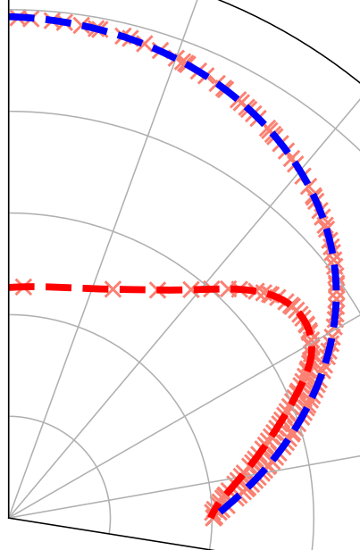
Comparison of model prediction and reference data for the bubble radius.
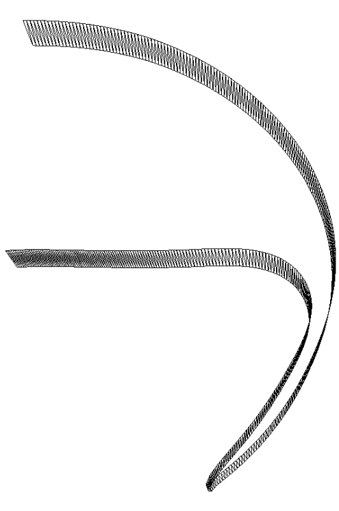
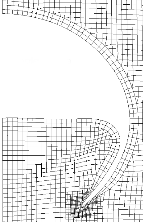
Mesh motion and zoom view of concentration boundary layer for $Re=569$ and $Sc=100$.

Global Sherwood number $Sh$ for two different mesh resolutions (3250 and 6500 cells/diameter). ~7h, serial, 2.4 GHz.
Outlook
What about unsupervised and reinforcement learning?
Extracting coherent flow structures
Modal decomp. = spatial structures + temp. behavior

spatial mode

temporal coefficient
Flow past a surface mounted cube at $Re=40000$.
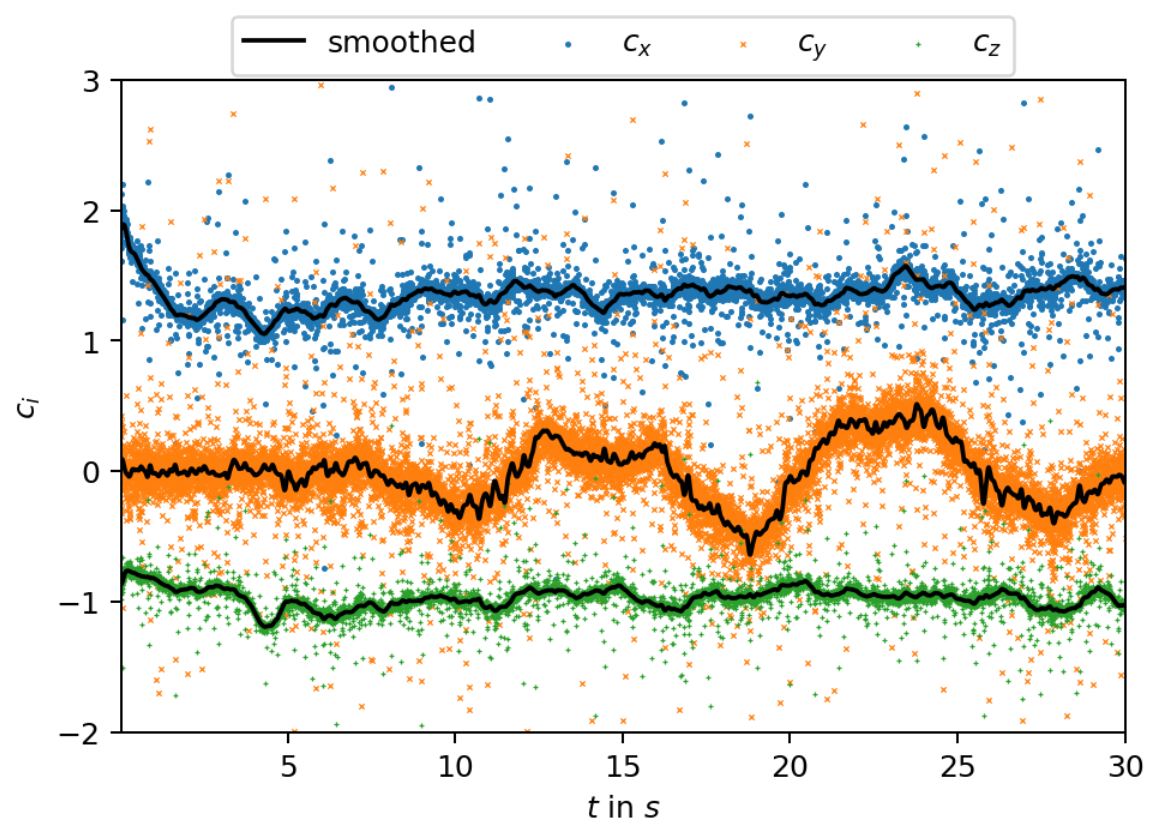
Forces acting in the cube expressed as force coefficients.
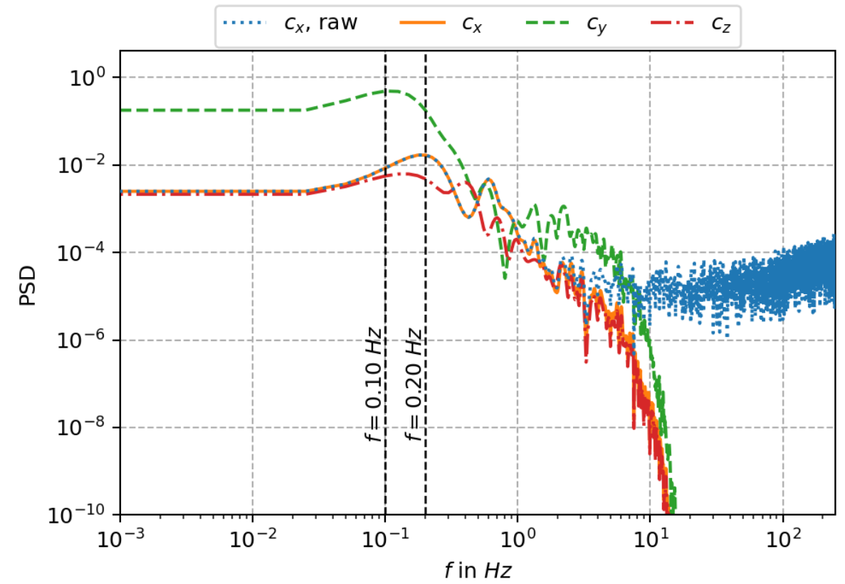
Power spectral density (PSD) of force coefficients.
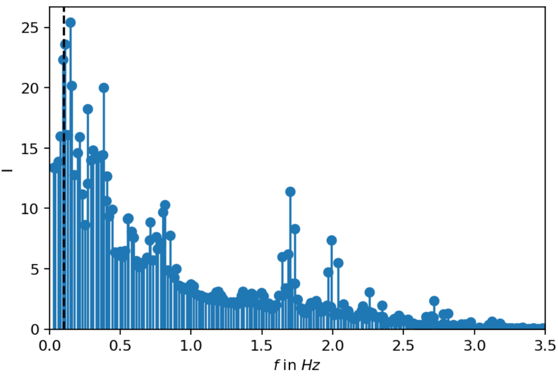
Spectrum of dynamic mode decomposition (DMD).
Reconstruction of main vortex shedding mode.
Reconstruction of high-frequency vortex shedding mode.
Closure modeling as a control problem
Closed-loop active flow control; variable inlet velocity/Reynolds number $Re(t) = 250 + 150\mathrm{sin}(\pi t)$; video by Fabian Gabriel.
LES with Smagorinsky model:
$$ \nu_t = (C_s \Delta)^2 \sqrt{2\tilde{S}_{ij}\tilde{S}_{ij}} $$
Kurz et al. (2022); $C_s$ - Smagorinsky constant; $\tilde{\mathbf{S}}$ - filtered strain rate tensor.
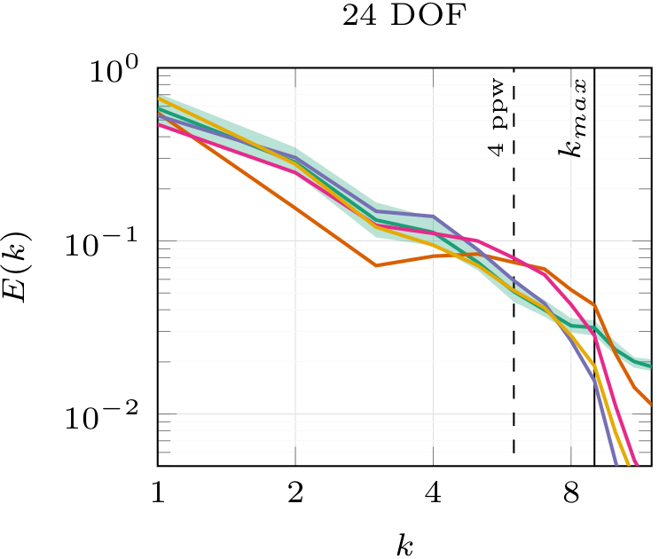
Energy spectra over wave number; DNS, DRL, SSM; Kurz et al. (2022).
Where to go from here:
- lecture resources: ML in CFD
- OpenFOAM SIG data-driven modeling
- reinforcement learning: drlFoam
- flowTorch documentation