Closed-loop active flow control (AFC)

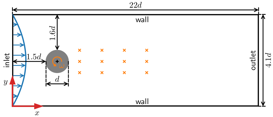
Flow past a cylinder in a narrow channel at $Re=\bar{U}_\mathrm{in}d/\nu = 100$.

Closed-loop control starts at $t=4s$.

motivation for closed-loop AFC

• (potentially) more efficient than open-loop control
• optimal control under changing conditions

How to design the control system?

$\rightarrow $ end-to-end optimization via simulations

Training cost DrivAer model

• $5$ hours/simulation (1000 MPI ranks)
• $10$ parallel simulations
• $100$ iterations $\rightarrow 20$ days turnaround time
• $20\times 24\times 10\times 1000 \approx 5\times 10^6 $ CPUh
• $0.01-0.05$ EUR/CPUh $\rightarrow 0.5-2$ mEUR

CFD simulations are expensive!

Proximal policy optimization (PPO)

Create an intelligent agent that learns to map states to actions such that expected returns are maximized.

experience tuple at step $n$ $$ (S_n, A_n, R_{n+1}, S_{n+1}) $$

trajectory over $N$ steps $$\tau = \left[ (S_0, A_0, R_1, S_1), \ldots ,(S_{N-1}, A_{N-1}, R_N, S_N)\right]$$

return - dealing with sequential feedback

$$ G_n = R_{n+1} + R_{n+2} + ... + R_N $$

learning what to expect in a given state - value function loss

$$ L_V = \frac{1}{N_\tau N} \sum\limits_{\tau = 1}^{N_\tau}\sum\limits_{n = 1}^{N} \left( V(S_n^\tau) - G_n^\tau \right)^2 $$

• $\tau$ - trajectory (single simulation)
• $S_n$ - state/observation (pressure)
• $V$ - parametrized value function
• clipping not included

Was the selected action a good one?

$$\delta_n = R_n + \gamma V(S_{n+1}) - V(S_n) $$ $$\delta_{n+1} = R_n + \gamma R_{n+1} + \gamma^2 V(S_{n+2}) - V(S_n) $$

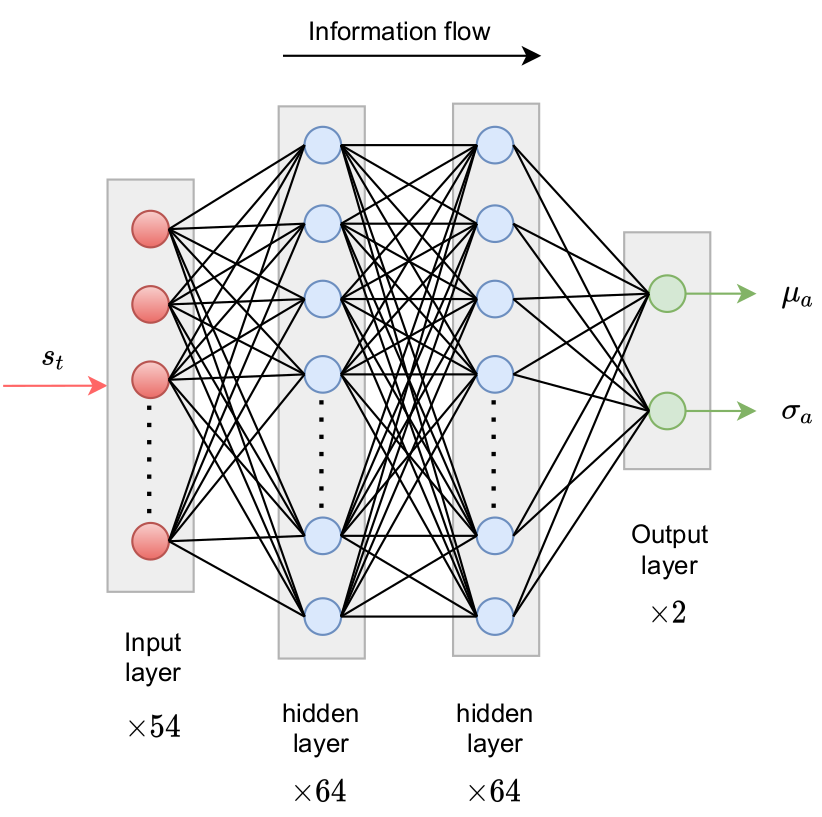
The policy network parametrizes a PDF over possible actions.

make good actions more likely - policy objective function

$$ J_\pi = \frac{1}{N_\tau N} \sum\limits_{\tau = 1}^{N_\tau}\sum\limits_{n = 1}^{N} \mathrm{min}\left[ \frac{\pi(A_n|S_n)}{\pi^{old}(A_n|S_n)} A^{GAE,\tau}_n, \mathrm{clamp}\left(\frac{\pi(A_n|S_n)}{\pi^{old}(A_n|S_n)}, 1-\epsilon, 1+\epsilon\right) A^{GAE,\tau}_n\right] $$

• $\pi$ - current policy
• $\pi^{old}$ - old policy (previous episode)
• entropy not included
• $J_\pi$ is maximized

Model ensemble PPO (MEPPO)

Idea: replace CFD with model(s) in some episodes

Challenge: dealing with surrogate model errors

for e in episodes:
    if not models_reliable():
        sample_trajectories_from_simulation()
        update_models()
    else:
        sample_trajectories_from_models()
    update_policy()
					

Based on Model Ensemble TRPO.

auto-regressive surrogate models with weights $\theta_m$

$$ m_{\theta_m} : (\underbrace{S_{n-d}, \ldots, S_{n-1}, S_n}_{\hat{S}_n}, A_n) \rightarrow (S_{n+1}, R_{n+1}) $$

How to sample from the ensemble?

1. pick initial sequence from CFD
2. generate model trajectories
   1. select random model
   2. sample action
   3. predict next state

When are the models reliable?

1. evaluate policy for every model
2. compare to previous policy loss
3. switch if loss did not decrease for
   at least $N_\mathrm{thr}$ of the models

Application: fluidic pinball

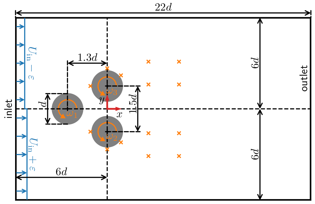
Fluidic pinball at $Re=\bar{U}_\mathrm{in}d/\nu = 100$; $\omega^\ast_i = \omega d/U_\mathrm{in} \in [-0.5, 0.5]$.

reward at step $n$

$$ c_x = \sum\limits_{i=1}^3 c_{x,i},\quad c_y = \sum\limits_{i=1}^3 c_{y,i} $$

$$ R_n = 1.5 - (c_{x,n} + 0.5 |c_{y,n}|) $$

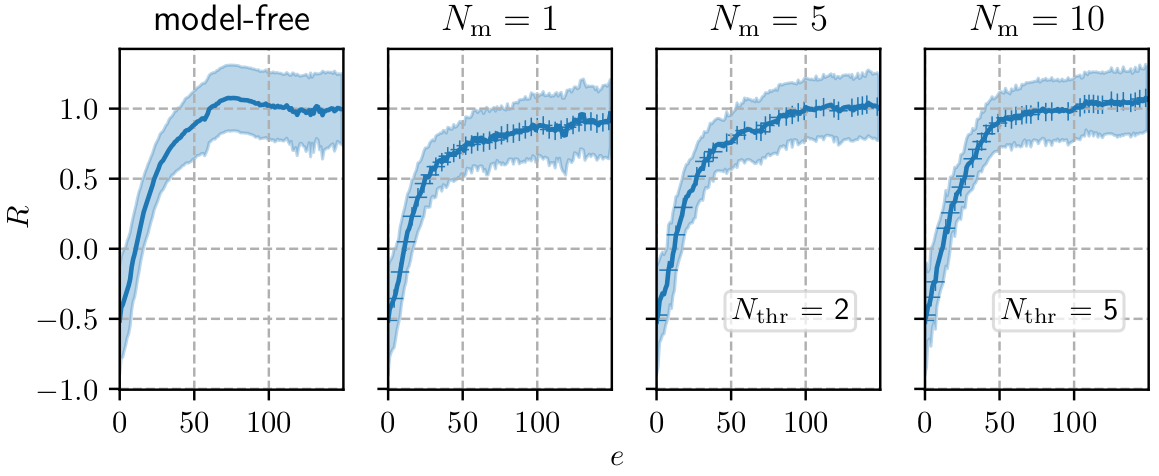
Mean reward $R$ per episode; $N_\mathrm{m}$ - ensemble size; $N_\mathrm{thr}$ - switching criterion.

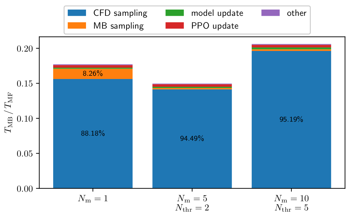
Composition of model-based training time $T_\mathrm{MB}$ relative to model-free training time $T_\mathrm{MF}$.

Closed-loop control starts at $t=200s$.

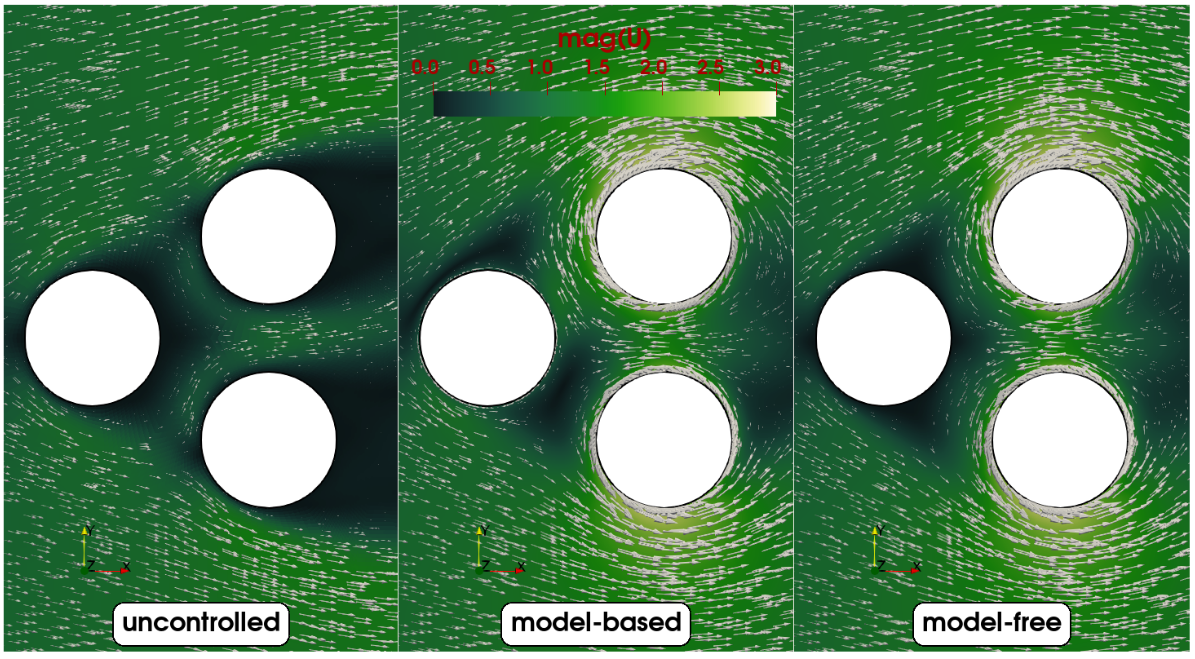
Snapshot of velocity fields (best policies).

Thank you for you attention!

Slides

GitHub