Active flow control via deep reinforcement learning implemented in OpenFOAM
Andre Weiner, Fabian Gabriel, Darshan Thummar, Richard Semaan
TU Braunschweig, Institute of Fluid
Mechanics
Outline
- Combining ML and CFD
- Deep reinforcement learning (DRL)
- Reinforcement learning (RL) basics
- Proximal policy optimization (PPO)
- DRL with OpenFOAM and PyTorch
- Where to go from here
Combining ML and CFD
why and how
Why combine CFD and ML?
CFD
- produces large amounts of complex data
- requires data or representations thereof
ML
- finds patterns in data
- creates useful representations of data
What is data?
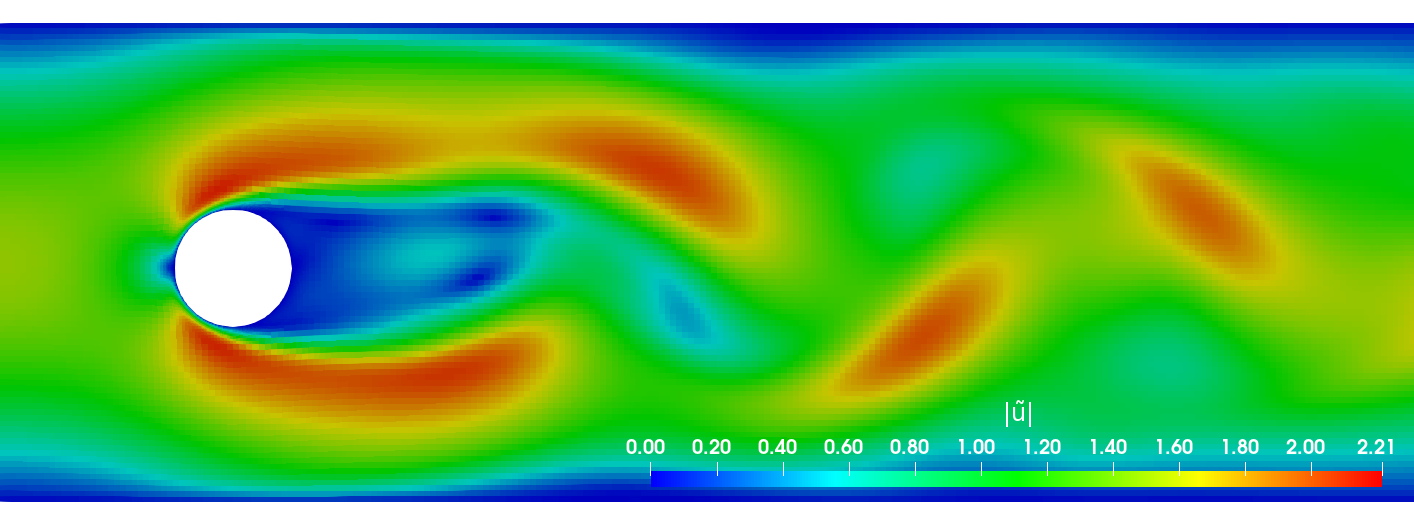
primary data: scalar/vector fields, boundary fields, integral values
# log.rhoPimpleFoam Courant Number mean: 0.020065182 max: 0.77497916 deltaT = 6.4813615e-07 Time = 1.22219e-06 PIMPLE: iteration 1 diagonal: Solving for rho, Initial residual = 0, Final residual = 0, No Iterations 0 DILUPBiCGStab: Solving for Ux, Initial residual = 0.0034181127, Final residual = 6.0056507e-05, No Iterations 1 DILUPBiCGStab: Solving for Uy, Initial residual = 0.0052004883, Final residual = 0.00012352706, No Iterations 1 DILUPBiCGStab: Solving for e, Initial residual = 0.06200185, Final residual = 0.0014223046, No Iterations 1 limitTemperature limitT Lower limited 0 (0%) of cells limitTemperature limitT Upper limited 0 (0%) of cells limitTemperature limitT Unlimited Tmax 329.54945 Unlimited Tmin 280.90821Checking geometry... ... Mesh has 2 solution (non-empty) directions (1 1 0) All edges aligned with or perpendicular to non-empty directions. Boundary openness (1.4469362e-19 3.3639901e-21 -2.058499e-13) OK. Max cell openness = 2.4668495e-16 OK. Max aspect ratio = 3.0216602 OK. Minimum face area = 7.0705331e-08. Maximum face area = 0.00033983685. Face area magnitudes OK. Min volume = 1.2975842e-10. Max volume = 6.2366859e-07. Total volume = 0.0017254212. Cell volumes OK. Mesh non-orthogonality Max: 60.489216 average: 4.0292071 Non-orthogonality check OK. Face pyramids OK. Max skewness = 1.1453509 OK. Coupled point location match (average 0) OK.
secondary data: log files, input dictionaries, mesh quality metrics, ...
Examples for data-driven workflows
Example: creating a surrogate or reduced-order model based on numerical data.
Example: creating a space and time dependent boundary condition based on numerical or experimental data.
Example: creating closure models based on numerical data.
Example: active flow control or shape optimization.
But how exactly does it work?
ML is not a generic problem solver ...
Supervised learning
Creating a mapping from features to labels based on examples.
Species transport around a rising bubble:
- simulation of two-phase flow dynamics
(specialized tool, not OpenFOAM) - ML models describing interface motion
- single phase simulations with species transport
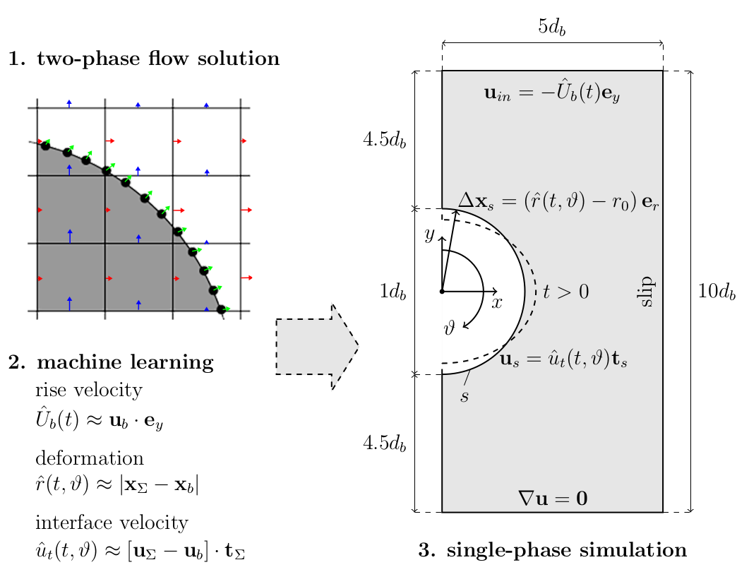
Mesh motion and zoom view of concentration boundary layer for $Re=569$ and $Sc=100$.
Unsupervised learning
Finding patterns in unlabeled data.
Dynamic mode decomposition (DMD):
Slice of local Mach number $Ma$, 3D, $\alpha=4^\circ$.
DMD buffet mode recon. based on slice of $u_x$.
What if my problem does not fit into these categories?
- break down problem into smaller junks
- mathematical, physical, numerical modeling
- combination of ML techniques
Reinforcement learning basics
(Deep) Reinforcement learning
Create an intelligent agent that learns to map states to actions such that cumulative rewards are maximized.
Experience tuple:
$$ \left\{ S_t, A_t, R_{t+1}, S_{t+1}\right\} $$
Trajectory:
$ \left\{S_0, A_0, R_1, S_1\right\} $
$ \left\{S_1, A_1, R_2, S_3\right\} $
$\left\{ ...\right\} $
Long-term consequences:
$$ G_t = \sum\limits_{l=0}^{N_t-t} \gamma^l R_{t+l} $$
- $t$ - control time step
- $G_t$ - discounted return
- $\gamma$ - discount factor, typically $\gamma=0.99$
- $N_t$ - number of control steps
Proximal policy optimization
Why PPO?
- continuous and discrete actions spaces
- relatively simple implementation
- restricted (robust) policy updates
- sample efficient
- ...
Refer to R. Paris et al. 2021 and the references therein for similar works employing PPO.
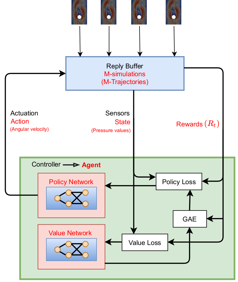
Proximal policy optimization (PPO) workflow (GAE - generalized advantage estimate).
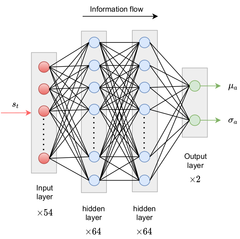
Policy network predicts probability density function(s) for action(s).
Comparison of Gauss and Beta distribution.
learning what to expect in a given state - value function loss
$$ L_V = \frac{1}{N_\tau N_t} \sum\limits_{\tau = 1}^{N_\tau}\sum\limits_{t = 1}^{N_t} \left( V(s_t^\tau) - G_t^\tau \right)^2 $$
- $\tau$ - trajectory (single simulation)
- $s_t$ - state/observation (pressure)
- $V$ - parametrized value function
- clipping not included
Was the selected action a good one?
$$\delta_t = R_t + \gamma V(s_{t+1}) - V(s_t) $$ $$ A_t^{GAE} = \sum\limits_{l=0}^{N_t-t} (\gamma \lambda)^l \delta_{t+l} $$
- $\delta_t$ - one-step advantage estimate
- $A_t^{GAE}$ - generalized advantage estimate
- $\lambda$ - smoothing parameter
make good actions more likely - policy objective function
$$ J_\pi = \frac{1}{N_\tau N_t} \sum\limits_{\tau = 1}^{N_\tau}\sum\limits_{t = 1}^{N_t} \left( \frac{\pi(a_t|s_t)}{\pi^{old}(a_t|s_t)} A^{GAE,\tau}_t\right) $$
- $\pi$ - current policy
- $\pi^{old}$ - old policy (previous episode)
- clipping and entropy not included
- $J_\pi$ is maximized
DRL with OpenFOAM and PyTorch
Active control of the flow past a cylinder
https://github.com/darshan315/flow_past_cylinder_by_DRL
https://github.com/FabianGabriel/Active_flow_control_past_cylinder_using_DRL
Flow past a circular cylinder at $Re=100$.
Things we might be interested in:
- reduce drag and lift forces
- mitigate extreme events
- maximize mixing in the wake
- ...
Can we reduce drag and lift forces?
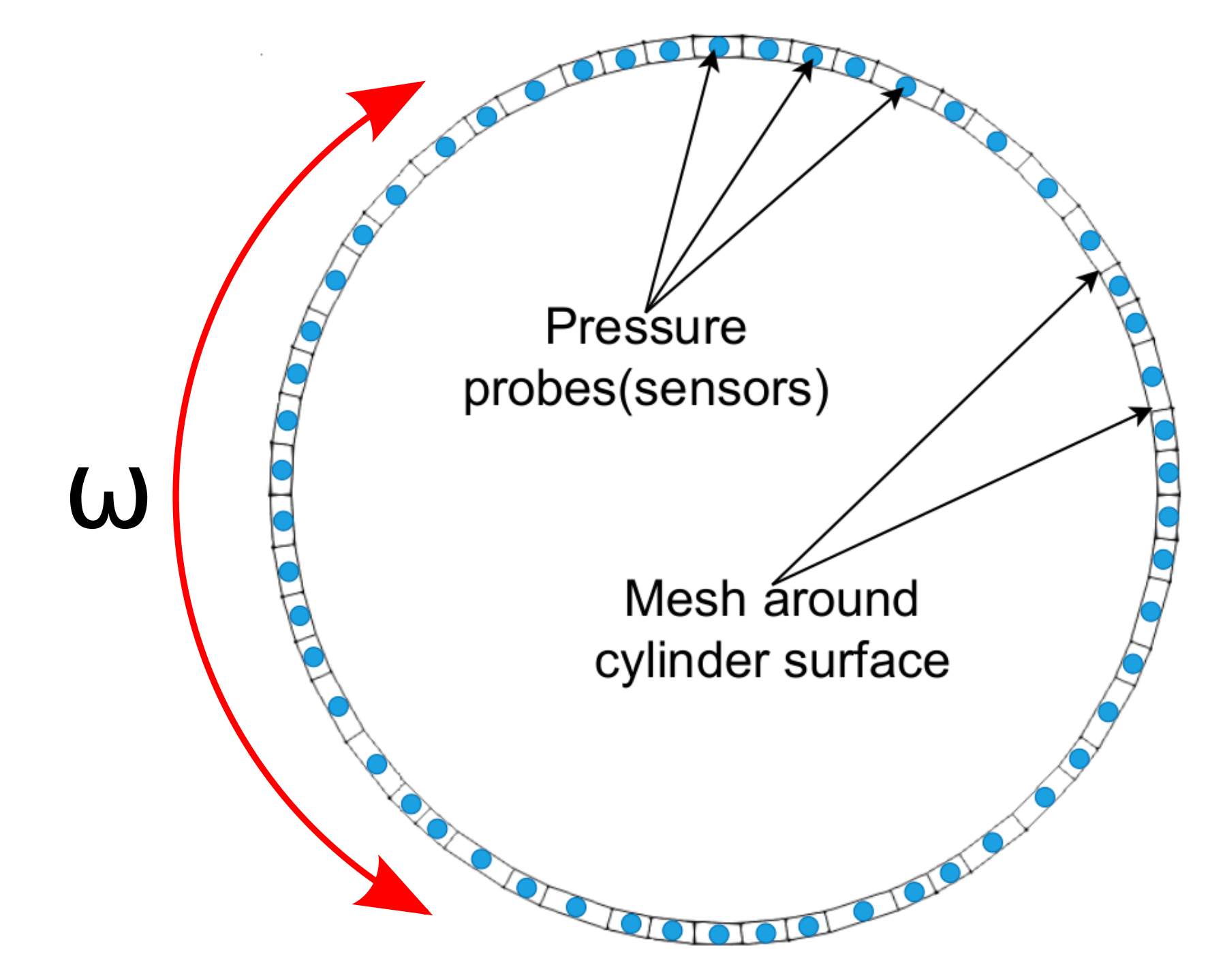
rewards - expressing the goal
$$ R_t = r_0 - \left( r_1 c_D + r_2 |c_L| \right) $$
- $c_D$ - drag coefficient
- $c_L$ - lift coefficient
- $r_i$ - constants
Python/PyTorch
- create policy and value networks
- fill trajectory buffer (run simulations)
- update policy and value networks
- go back to 1. until converged
Implementation follows closely chapter 12 of Miguel Morales's Grokking Deep Reinforcement Learning
C++/OpenFOAM/PyTorch
- read policy network
- sample and apply action
- write trajectory (experience tuples)
Boundary condition defined in 0/U
cylinder
{
	type            agentRotatingWallVelocity;
	// center of cylinder
	origin          (0.2 0.2 0.0);
	// axis of rotation; normal to 2D domain
	axis            (0 0 1);
	// name of the policy network; must be a torchscript file
	policy          "policy.pt";
	// when to start controlling
	startTime       0.01;
	// how often to evaluate policy
	interval        20;
	// if true, the angular velocity is sampled from a Gaussian distribution
	// if false, the mean value predicted by the policy is used
	train           true;
	// maximum allowed angular velocity
	absOmegaMax     0.05;
}
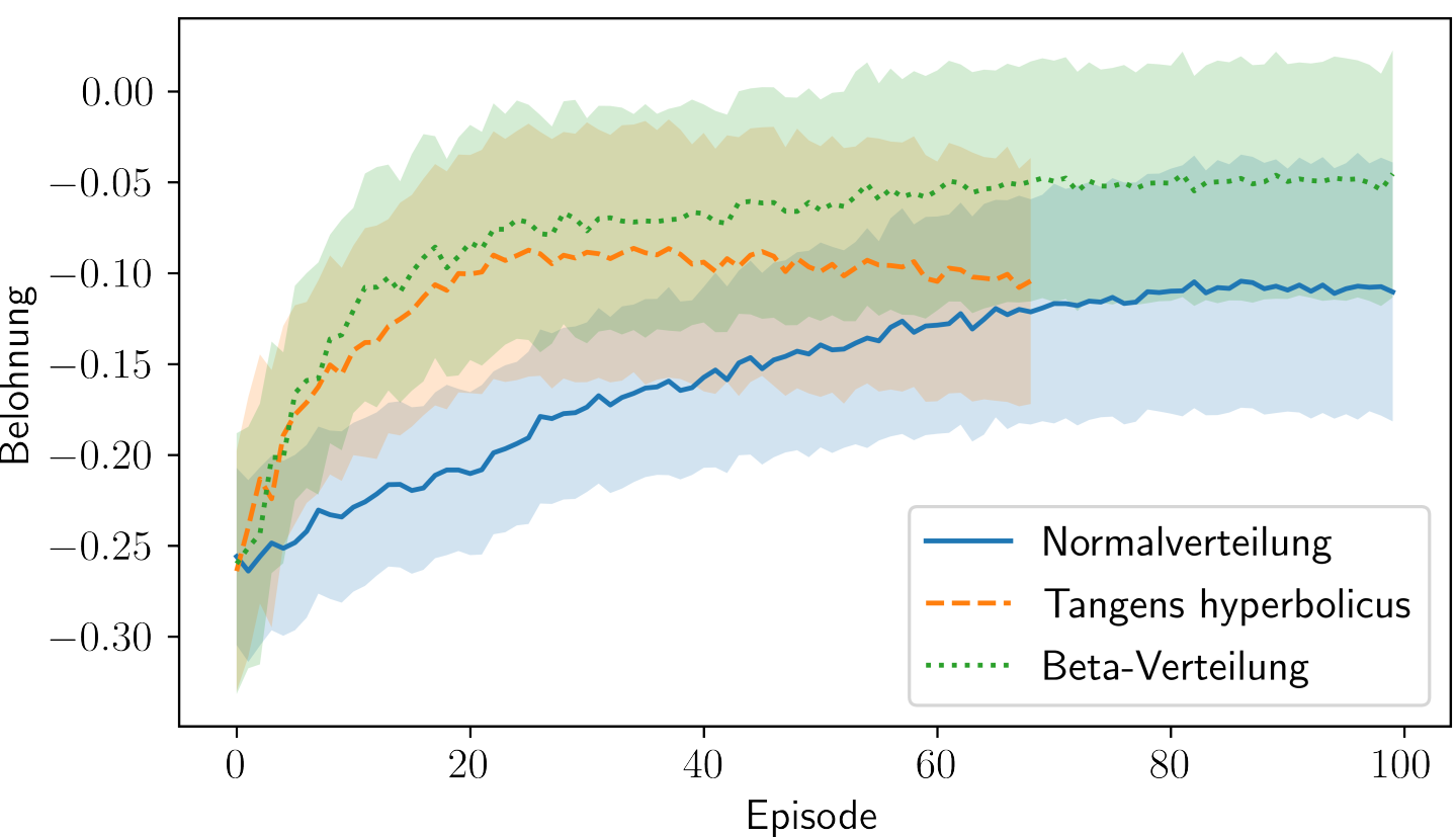
Cumulative rewards vs. episodes for various distributions.
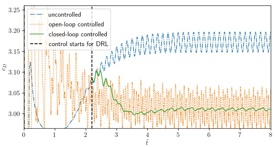
Comparison of uncontrolled, open-loop controlled, and closed-loop controlled drag.
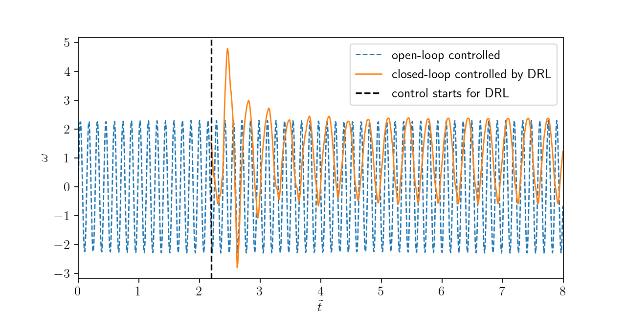
Angular velocity for open and closed-loop control.
How robust is the controller?
- training with steady inlet velocity
$Re=\{100, 200, 400 \}$ - test with unsteady inlet velocity
$Re(t)= 250 + 150\mathrm{sin}(\pi t)$
Variable inlet velocity/Reynolds number $Re(t) = 250 + 150\mathrm{sin}(\pi t)$
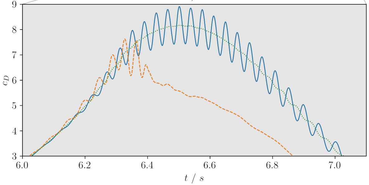
Drag coefficient for transient inlet velocity: uncontrolled and controlled.
Where to go from here
Data-driven modeling SIG
- OpenFOAM wiki (overview)
- Github (resource aggregation)
- Upcoming meeting: June 9, 2022
Lecture on ML in CFD
- covers all types of ML
- freely available on Github
- work in progress
THE END
Thank you for you attention!
