Model-based deep reinforcement learning for flow control
Andre Weiner, Janis Geise
TU Braunschweig, Institute of Fluid
Mechanics
Outline
- Closed-loop active flow control
- Proximal policy optimization (PPO)
- Model-based PPO
Closed-loop active flow control
Goals of flow control:
- drag reduction
- load reduction
- process intensification
- noise reduction
- ...
Categories of flow control:
- passive: geometry, fluid properties, ...
- active: blowing/suction, heating/cooling, ...
energy input vs. efficiency gain
Categories of active flow control:
- open-loop: actuation predefined
- closed-loop: actuation based on sensor input
How to find the control law?
Closed-loop flow control with variable Reynolds number; source: F. Gabriel 2021.
Why CFD-based DRL?
- save virtual environment
- prior optimization, e.g., sensor placement
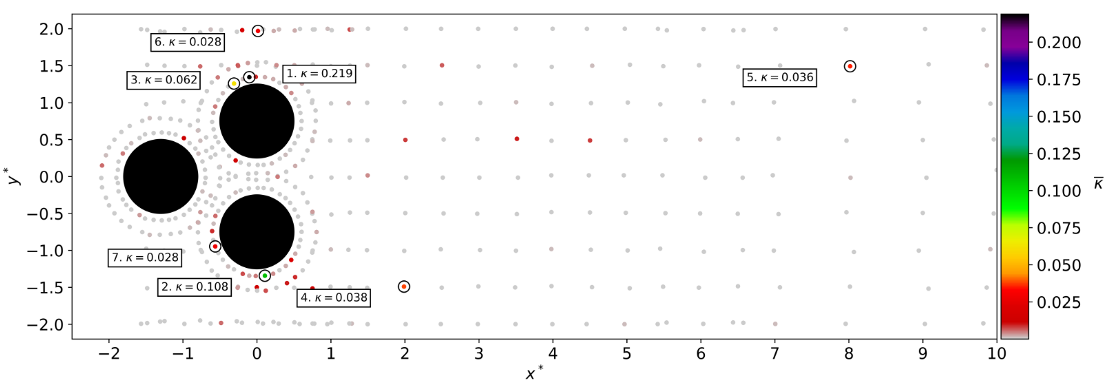
Time-averaged attention weights $\bar{\kappa}$
Tom Krogmann 10.5281/zenodo.7636959
Training cost DrivAer model
- $8$ hours/simulation (2000 MPI ranks)
- $10$ parallel simulations
- $3$ episodes/day
- $60$ days/training (180 episodes)
- $60\times 24\times 10\times 2000 \approx 30\times 10^6 $ core hours
CFD environments are expensive!
Proximal policy optimization

Create an intelligent agent that learns to map states to actions such that expected returns are maximized.
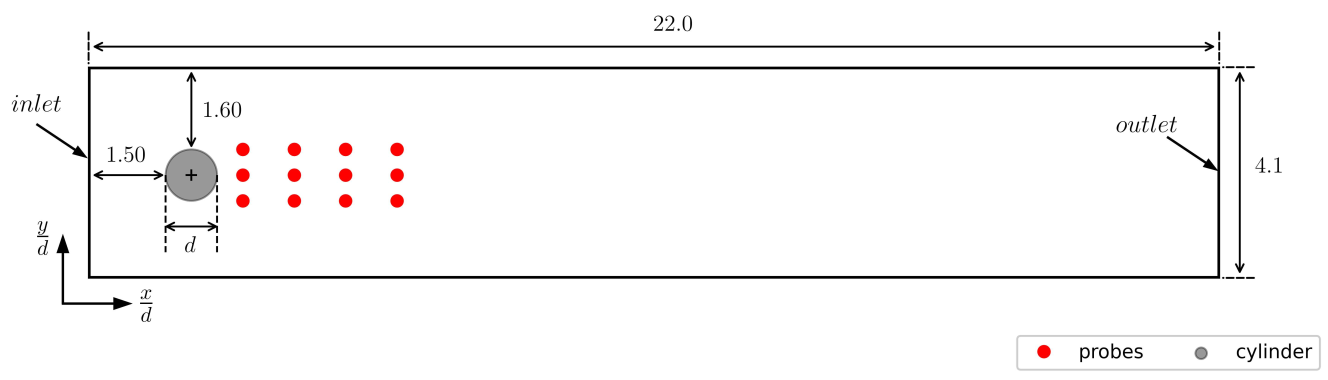
Flow past a cylinder benchmark.
What is our goal?
$r=3-(c_d + 0.1 |c_l|)$
$c_d$, $c_l$ - drag and lift coeff.; see J. Rabault et al.
Long-term consequences:
$$ G_t = \sum\limits_{l=0}^{N_t-t} \gamma^l R_{t+l} $$
- $t$ - control time step
- $G_t$ - discounted return
- $\gamma$ - discount factor, typically $\gamma=0.99$
- $N_t$ - number of control steps
What to expect in a given state?
$$ L_V = \frac{1}{N_\tau N_t} \sum\limits_{\tau = 1}^{N_\tau}\sum\limits_{t = 1}^{N_t} \left( V(s_t^\tau) - G_t^\tau \right)^2 $$
- $\tau$ - trajectory (single simulation)
- $s_t$ - state/observation (pressure)
- $V$ - parametrized value function
- clipping not included
Was the selected action a good one?
$$\delta_t = R_t + \gamma V(s_{t+1}) - V(s_t) $$ $$ A_t^{GAE} = \sum\limits_{l=0}^{N_t-t} (\gamma \lambda)^l \delta_{t+l} $$
- $\delta_t$ - one-step advantage estimate
- $A_t^{GAE}$ - generalized advantage estimate
- $\lambda$ - smoothing parameter
Making good actions more likely:
$$ J_\pi = \frac{1}{N_\tau N_t} \sum\limits_{\tau = 1}^{N_\tau}\sum\limits_{t = 1}^{N_t} \left( \frac{\pi(a_t|s_t)}{\pi^{old}(a_t|s_t)} A^{GAE,\tau}_t\right) $$
- $\pi$ - current policy
- $\pi^{old}$ - old policy (previous episode)
- clipping and entropy not included
- $J_\pi$ is maximized
Model-based PPO
Janis Geise, Github, 10.5281/zenodo.7642927
Idea: replace CFD with model(s) in some episodes
for e in episodes:
    if models_reliable():
        sample_trajectories_from_models()
    else:
        sample_trajectories_from_simulation()
        update_models()
    update_policy()
Based on Model Ensemble TRPO.
When are the models reliable?
- evaluate policy for every model
- compare to previous policy loss
- switch if loss did not decrease for
at least $50\%$ of the models
How to sample from the ensemble?
- pick initial sequence from CFD
- fill buffer
- select random model
- sample action
- predict next state
Recipe to create env. models:
- input/output normalization
- fully-connected, feed-forward
- time delays (~30)
- layer normalization
- batch training (size ~100)
- learning rate decay (on plateau)
- "early stopping"
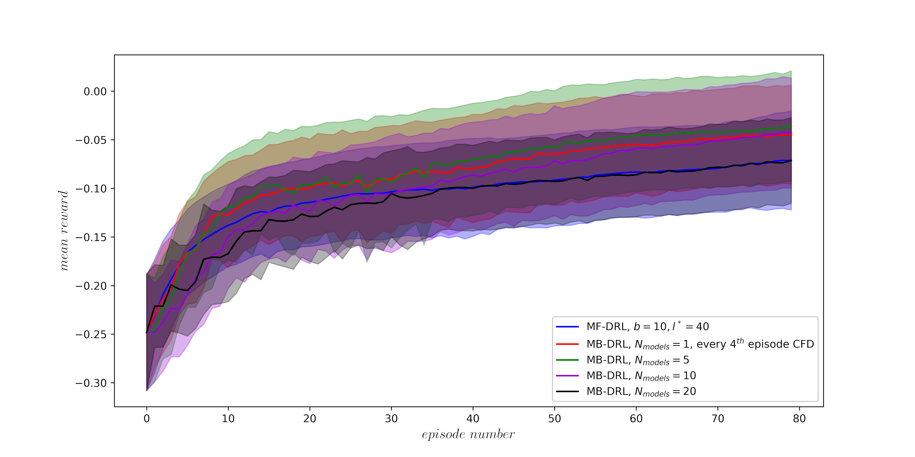
Influence on the number of models; average over trajectories and 3 seeds.
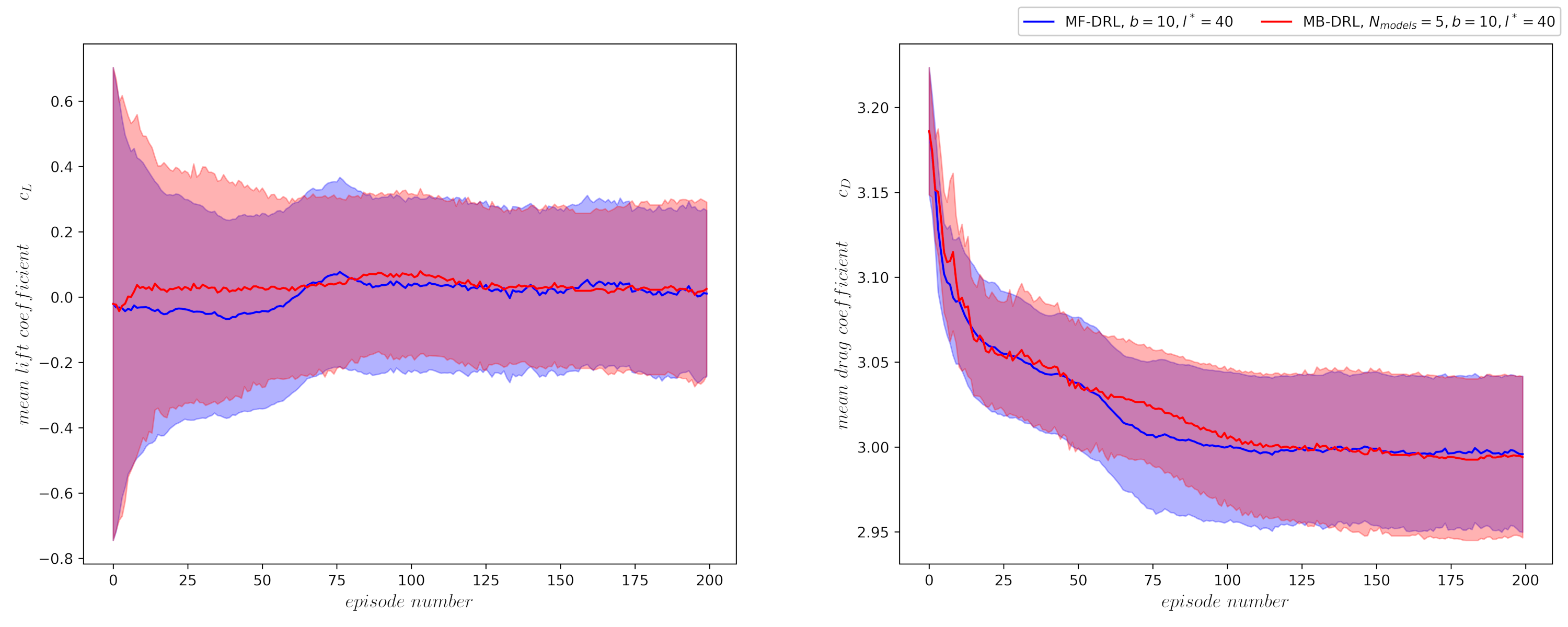
Comparison of best policy over 3 seeds.
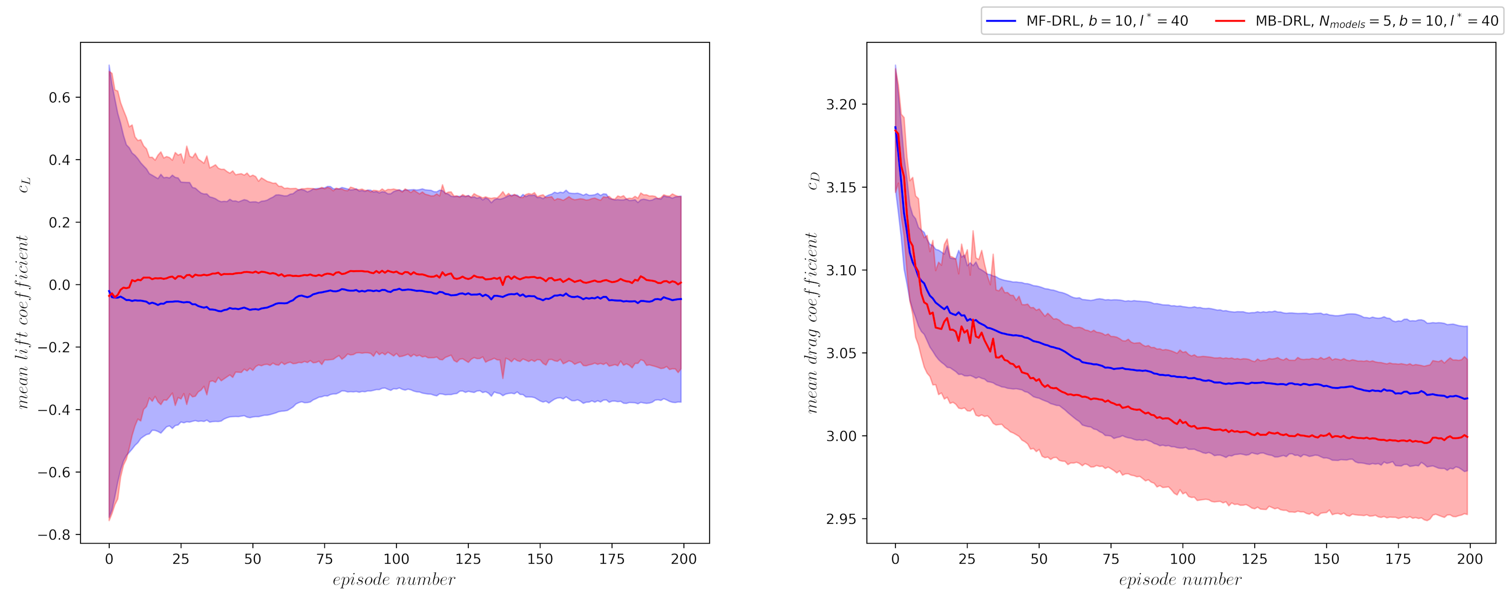
Average performance over 3 seeds.
What are the savings?
$50-70\%$ in training time