Introduction to machine learning
Andre Weiner
TU Dresden, Institute of fluid mechanics, PSM

These slides and most
of the linked resources are licensed under a
Creative Commons Attribution 4.0
International License.
Last lectures
The finite volume method in a nutshell
- Mathematical model
- Domain discretization (meshing)
- Equation discretization
- Solving the linear system of equations
- OpenFOAM and Basilisk
Outline
Introduction to selected ML concepts
- Floating point numbers
- Exploring parameter spaces
- Generating data with simulations
- Normalizing data
- Feature selection and design
- Deep learning
Floating point numbers
IEEE 754 standard
Floating point number representation:
$$ S\times M\times 2^{E-e} $$- $S$ - sign, $M$ - mantissa, $E$ - exponent
- $e$ - machine constant
- typically 32 or 64 bit (4 or 8 bytes)
How are bits distributed among $S$, $M$, $E$?
for dtype in [np.float32, np.float64]:
	finfo = np.finfo(dtype)
	print(f"dtype: {finfo.dtype}")
	print(f"Number of bits: {finfo.bits}")
	print(f"Bits reserved for mantissa: {finfo.nmant}")
	print(f"Bits reserved for exponent: {finfo.iexp}")
# output
dtype: float32
Number of bits: 32
Bits reserved for mantissa: 23
Bits reserved for exponent: 8
# ----------------------------
dtype: float64
Number of bits: 64
Bits reserved for mantissa: 52
Bits reserved for exponent: 11
Exercise: represent 85.125 as 32 bit float.
Which numbers can we represent?
for dtype in [np.float32, np.float64]:
	finfo = np.finfo(dtype)
	print("Largest representable number: {:e}".format(finfo.max))
	print("Smallest representable number: {:e}".format(finfo.min))
	print("Machine tolerance: {:e}".format(finfo.eps))
	print(f"Approximately accurate up to {finfo.precision} decimal digits")
# output
Largest representable number: 3.402823e+38
Smallest representable number: -3.402823e+38
Machine tolerance: 1.192093e-07
Approximately accurate up to 6 decimal digits
# -------------------------------------------
Largest representable number: 1.797693e+308
Smallest representable number: -1.797693e+308
Machine tolerance: 2.220446e-16
Approximately accurate up to 15 decimal digits
Can I represent 123'456'789 as 32 bit float?
What is the preferred floating point type in
- CFD?
- ML?
- DL?
Setting the default floating point type in PyTorch:
x = pt.tensor(1.0)
print(x.dtype)
pt.set_default_dtype(pt.float64)
x = pt.tensor(1.0)
print(x.dtype)
# expected output
torch.float32
torch.float64
What is the machine tolerance?
Experiment: adding a small number to one
a = pt.tensor(1.0, dtype=pt.float32)
for b in [10**i for i in range(-1, -11, -1)]:
    print("1.0 + {:1.1e} = {:10.10f}".format(b, a+b))
# output
# for readability 0123456789
1.0 + 1.0e-01 = 1.1000000238
1.0 + 1.0e-02 = 1.0099999905
1.0 + 1.0e-03 = 1.0010000467
1.0 + 1.0e-04 = 1.0001000166
1.0 + 1.0e-05 = 1.0000100136
1.0 + 1.0e-06 = 1.0000009537
1.0 + 1.0e-07 = 1.0000001192
1.0 + 1.0e-08 = 1.0000000000
1.0 + 1.0e-09 = 1.0000000000
1.0 + 1.0e-10 = 1.0000000000
How is this type of error referred to?
Task: fit a 4th order polynomial
$$ y(x) = ax^4+bx^3+cx^2+dx+e $$to data with $-0.01 \le x \le 0.01$ and $1 \le y \le 10$.
Problems?
Roundoff errors affect you sooner than you think!
for x in pt.arange(-0.01, 0.011, 0.0025):
    print("x={:+1.4e}, x**2={:1.4e}, x**3={:+1.4e}, x**4={:1.4e}".format(x, x**2, x**3, x**4))
# expected output
x=-1.0000e-02, x**2=1.0000e-04, x**3=-1.0000e-06, x**4=1.0000e-08
x=-7.5000e-03, x**2=5.6250e-05, x**3=-4.2187e-07, x**4=3.1641e-09
x=-5.0000e-03, x**2=2.5000e-05, x**3=-1.2500e-07, x**4=6.2500e-10
x=-2.5000e-03, x**2=6.2500e-06, x**3=-1.5625e-08, x**4=3.9062e-11
x=+0.0000e+00, x**2=0.0000e+00, x**3=+0.0000e+00, x**4=0.0000e+00
x=+2.5000e-03, x**2=6.2500e-06, x**3=+1.5625e-08, x**4=3.9062e-11
x=+5.0000e-03, x**2=2.5000e-05, x**3=+1.2500e-07, x**4=6.2500e-10
x=+7.5000e-03, x**2=5.6250e-05, x**3=+4.2187e-07, x**4=3.1641e-09
x=+1.0000e-02, x**2=1.0000e-04, x**3=+1.0000e-06, x**4=1.0000e-08
Another experiment:
a = pt.tensor(1.0)
print("a={:1.10f}".format(a))
b = a - 2.0/3.0
print("b={:1.10f}".format(b))
a = 3.0*b
print("a={:1.10f}".format(a))
# expected output
a=1.0000000000
b=0.3333333135
a=0.9999999404
Where does the error come from?
Roundoff errors accumulate!
def iterate(n_iter: float = 1):
    a = pt.tensor(1.0)
    for _ in range(n_iter):
        b = a - 2/3
        a = 3.0 * b
    print(f"a={a:1.10f} after {n_iter:1d} iteration(s)")

for i in range(1, 10):
    iterate(i)
# expected output
a=0.9999999404 after 1 iteration(s)
a=0.9999997616 after 2 iteration(s)
a=0.9999992251 after 3 iteration(s)
a=0.9999976158 after 4 iteration(s)
a=0.9999927878 after 5 iteration(s)
a=0.9999783039 after 6 iteration(s)
a=0.9999348521 after 7 iteration(s)
a=0.9998044968 after 8 iteration(s)
a=0.9994134307 after 9 iteration(s)
Truncation error
Results from discrete approximations of continuous variables.
$$ \int\limits_0^1 x^2 \mathrm{d}x = 1/3 $$Cannot be avoided even with perfectly accurate floating point numbers.
Truncation error of the trapezoidal rule with increasing number of integration steps.
What is the (typical) convergence order of OpenFOAM and Basilisk?
Exploring parameter spaces
Sampling a parameter space may be expensive, so drawing samples should be:
- efficient - not more samples then necessary
- homogeneous - good coverage of the entire space
- unbiased$^*$ - equal sampling probability for all points
$^*$ assuming there is no prior knowledge about the parameter space
Task: establish relation between $Re$ and $c_d$; assumptions:
- no prior knowledge of dependency
- lower bound $Re=10$
- upper bound $Re=100$
- $N_s = 10$ simulation are affordable
How do we draw the samples?
Equally spaced samples:
$Re = \{10, 20, 30, ..., 100 \}$
- unbiased?
- homogeneous?
- efficient?
Effect of bias on sampling.
How does the number of required samples $N_t$ scale with the number of parameters $d$ if we treat all parameters equally?
- linearly: $N_t = N_s d$
- quadratically: $N_t = N_s d^2$
- exponentially: $N_t = N_s^d$
Randomly drawn samples:
$Re = \{51, 45, 91, 84, 92, 67, 99, 71, 100, 41 \}$
- unbiased?
- homogeneous?
- efficient?
Combining advantages: latin hypercube sampling (LHS)
- segment parameter space in $N_s$ equally sized junks (hypercubes)
- randomly draw one sample in each segment of each parameter
- shuffle and combine samples
LHS sampling in Python/PyTorch
def lhs_sampling(x_min: list, x_max: list, n_samples: int) -> pt.Tensor:
	assert len(x_min) == len(x_max)
	n_parameters = len(x_min)
	samples = pt.zeros((n_parameters, n_samples))
	for i, (lower, upper) in enumerate(zip(x_min, x_max)):
		bounds = pt.linspace(lower, upper, n_samples+1)
		rand = bounds[:-1] + pt.rand(n_samples) * (bounds[1:]-bounds[:-1])
		samples[i, :] = rand[pt.randperm(n_samples)]
	return samples
Generating data from simulations
Requirements for a good base simulation:
- setup reflects mathematical problem
- low mesh dependency
- validated against reference data
- setup is optimized
Task: study dependency of vortex shedding frequency on Reynolds number for the flow past a cylinder; $80 < Re < 1000$.
Mesh dependency study for
- all cases
- lowest $Re$
- largest $Re$
- random $Re$ (unbiased)
In the individual simulation setups, do we have to change only $Re$?
sed - Stream EDitor: replace text in files
sed -i 's/old_text/new_text/' exampleDict
Running external programs with system and Popen:
# with os.system
cmd = "sed -i 's/old_text/new_text/' exampleDict"
os.system(cmd)
# with subprocess.Popen
cmd = ["sed", "-i", "'s/old_text/new_text/'", "exampleDict"]
p = subprocess.Popen(cmd, cwd="./test_case/")
# print exit code to check if execution was successful
print(p.poll())
Leveraging the hardware's full potential:
def run_simulation(path: str):
    return_code = Popen(["./Allrun"], cwd=path).wait()
    if return_code == 0:
        print(f"Simulation {path} completed successfully.")
    else:
        print(f"Warning: simulation {path} failed.")

simulations = ["./sim_0/", "./sim_1/", "./sim_2/"]
pool = Pool(2)  # from multiprocessing
with pool:
    pool.map(run_simulation, simulations)
Normalizing data
Example dataset with Reynolds $Re$ number, angle of attack $\alpha$, and lift coefficient $c_l$:
- $10\times 10^6 < Re < 20\times 10^6$
- $0^\circ < \alpha < 4^\circ$
- $c_l$ - measured
Avoiding roundoff errors: min-max-normalization for each feature/label $x_i$:
$$ x_i^* = \frac{x_i - x_{i,min}}{x_{i,max}-x_{i,min}},\quad x_i^*\in [0,1] $$ $$ \tilde{x}_i = 2x_i^* - 1,\quad \tilde{x}_i \in [-1,1] $$Avoiding roundoff errors: mean-std.-normalization for each feature/label $x_i$:
$$ x_i^* = \frac{x_i - \mu_{x_i}}{\sigma_{x_i}} $$- $\mu_{x_i}$ - mean
- $\sigma_{x_i}$ - standard deviation
- less sensitive to outliers
Sigmoid function $\sigma (x) = 1/(1+e^{-x})$.
Intuitively, how would you group the measurements?
- 1+2, 3
- 1+3, 2
- 2+3, 1
Feature selection and design
Feature design
- some features are naturally given
- additional features may be designed to
- embed mathematical constraints
- embed known physical laws
- decrease variance
Rule of thumb: extract/generate as many features as possible.
Features must be available in the target application!
Feature selection tools
- correlation (heatmap)
- sequential forward/backward selection
- random feature permutation
- attention (DL)
- ...

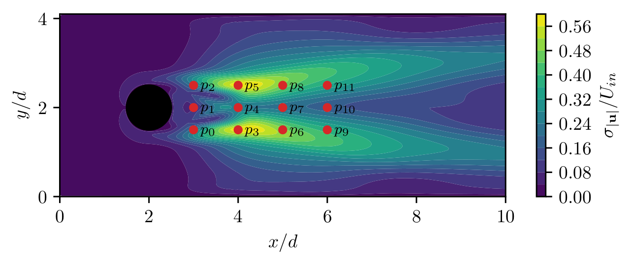
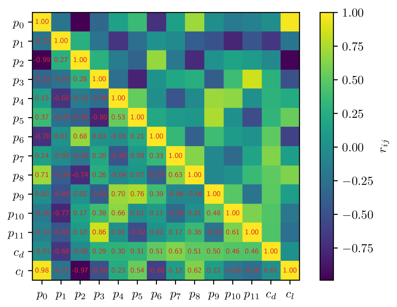
Question: which sensors are suitable for drag/lift prediction?

Example for correlation heatmap.
Automated feature selection/learning:
- sequential forward/backward selection
- random feature permutation
- attention (learned feature importance)
Deep learning
- test case overview
- simple feed-forward networks
- preparing the datasets
- generic training loop
- more building blocks
- dealing with uncertainty
- visualizing prediction errors
Test case overview
- 1D setup for computing channel flow (exercise)
- 16 simulations with varying inlet velocity $\bar{U}$
- Reynolds number $Re = 2\bar{U}\delta/\nu$
- data: streamwise velocity component $u_x$ for varying distances normal to wall $y$
Goal: model for streamwise velocity
$$ \tilde{u}_{x} = f_{\mathbf{\theta}}(\tilde{y}, Re) $$$\tilde{u}_{x} = u_x/\bar{U}_{max}$, $\tilde{y} = y/(2\delta)$
Streamwise velocity component for various $Re$.
Simple feed-forward networks
Assumptions for this lecture:
- only fully connected layers
- constant number of neurons for each hidden layer
- blind usage as generic function approximation tool
Terminology
Feature and label vectors
$N_s$ samples of $N_f$ features and $N_l$ labels
| $i$ | $x_{1}$ | ... | $x_{N_f}$ | $y_{1}$ | ... | $y_{N_l}$ |
|---|---|---|---|---|---|---|
| 1 | 0.1 | ... | 0.6 | 0.5 | ... | 0.2 |
| ... | ... | ... | ... | ... | ... | ... |
| $N_s$ | 1.0 | ... | 0.7 | 0.4 | ... | 0.2 |
ML models often map multiple inputs to multiple outputs!
Feature vector:
$$ \mathbf{x} = \left[x_{1}, x_{2}, ..., x_{N_f}\right]^T $$ $\mathbf{x}$ - column vector of length $N_f$
$$ \mathbf{X} = \left[\mathbf{x}_{1}, \mathbf{x}_{2}, ..., \mathbf{x}_{N_s}\right] $$ $\mathbf{X}$ - matrix with $N_s$ rows and $N_f$ columns
Label vector:
$$ \mathbf{y} = \left[y_{1}, y_{2}, ..., y_{N_l}\right]^T $$ $\mathbf{y}$ - column vector of length $N_l$
$$ \mathbf{Y} = \left[\mathbf{y}_{1}, \mathbf{y}_{2}, ..., \mathbf{y}_{N_s}\right] $$ $\mathbf{Y}$ - matrix with $N_s$ rows and $N_l$ columns
ML model and prediction
$$ f_\mathbf{\theta}(\mathbf{x}) : \mathbb{R}^{N_f} \rightarrow \mathbb{R}^{N_l} $$ $f_\mathbf{\theta}$ - ML model with weights $\mathbf{\theta}$ mapping from the feature space $\mathbb{R}^{N_f}$ to the label space $\mathbb{R}^{N_l}$ $$ \hat{\mathrm{y}}_i = f_\mathbf{\theta}(\mathbf{x}_i) $$ $\hat{\mathrm{y}}_i$ - (model) prediction

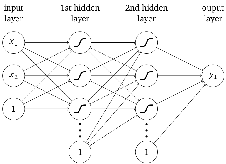
- neuron: weighted sum + nonlinear map
- lines: weights/free parameters
- input/output: features/labels
- 1: bias unit
Formalization: weighted sum of inputs
$$ z_j^l\left(\mathbf{x}^{l-1}\right) = \sum\limits_{i=1}^{N_{neu}^{l-1}} w_{ji}^{l-1} x_i^{l-1} + b_j^{l-1} $$- $l$ - current layer
- $N_{neu}$ - neurons per layer
- $\mathbf{x}$ - feature/input
- $\mathbf{W}$ - weight matrix
Vector notation:
$$ \mathbf{z}_l = \mathbf{W}_{l-1}^T \mathbf{x}_{l-1} + \mathbf{b}_{l-1}, $$
Formalization: nonlinear map/activation
$$ \mathbf{x}_l = a_l(\mathbf{z}_l) = a_l(\mathbf{W}_{l-1}^T\mathbf{x}_{l-1}+\mathbf{b}_{l-1}). $$- $a_l$ - activation function
- $\mathbf{z}_l$ - weighted sum
- $l$ - current layer
Example: network with two hidden layers
$$ f_\theta(\mathbf{x}) = \mathbf{W}_2^T a_1(\mathbf{W}_1^T a_0(\mathbf{W}_0^T\mathbf{x} + \mathbf{b}_0) + \mathbf{b}_1) + \mathbf{b}_2, $$Short reminder - function composition:
- $f(x) = 2x+1$
- $g(x) = x^2$
- $h(x) = f(g(x)) = f \circ g(x) = 2x^2+1$
Formalization: layer composition
$$ f_{\theta}(\mathbf{x}) = m_{N_L} \circ m_{N_{L-1}}\circ ... \circ m_0 (\mathbf{x}), $$$N_L$ - number of layers
Preparing the dataset
def reshape_data(u_x_norm, y_norm, Re) -> pt.Tensor:
    data = pt.zeros((u_x_norm.shape[0]*u_x_norm.shape[1], 3))
    for i in range(u_x_norm.shape[1]):
        start, end = i*u_x_norm.shape[0], (i+1)*u_x_norm.shape[0]
        data[start:end, 0] = u_x_norm[:, i]
        data[start:end, 1] = y_norm
        data[start:end, 2] = Re[i]
    return data
Additional step: normalization!
Splitting the data
- training data: optimization of model weights
- validation data: sanity check during training
- testing data: final performance evaluation
Splitting the data
n_Re = len(Re)
probs = pt.ones(u_x.shape[-1])
probs[0] = 0.0
probs[-1] = 0.0
train_size, val_size, test_size = 8, 3, 3
test_idx = pt.multinomial(probs, test_size)
probs[test_idx] = 0.0
val_idx = pt.multinomial(probs, val_size)
probs[val_idx] = 0.0
train_idx = pt.multinomial(probs, train_size)
train_idx = pt.cat((train_idx, pt.tensor([0, n_Re-1], dtype=pt.int64)))
The PyTorch dataloader
train_loader = pt.utils.data.DataLoader(train_dataset, batch_size=500, shuffle=True)
	for features, labels in train_loader:
		print(features.shape, labels.shape)
	# expected output
	torch.Size([500, 2]) torch.Size([500, 1])
	torch.Size([500, 2]) torch.Size([500, 1])
	...
A generic training loop
Mean squared error loss function:
$$ L_2(\mathbf{\theta}) = \frac{1}{N_s}\sum\limits_{i=1}^{N_s} \left( \mathbf{y}_i - f_{\mathbf{\theta}}(\mathbf{x}_i) \right)^2 $$
Optimization problem:
$$ \mathbf{\theta}^\ast = \underset{\mathbf{\theta}}{\mathrm{argmin}} L_2 (\mathbf{\theta}) $$
Gradient decent update rule:
$$ \mathbf{\theta}_{n+1} = \mathbf{\theta}_n - \lambda_0 \frac{\mathrm{d}L}{\mathrm{d}\mathbf{\theta}} $$
More complex update rule:
$$ \mathbf{\theta}_{n+1} = \mathbf{\theta}_n - g\left(\lambda_0,\frac{\mathrm{d}L}{\mathrm{d}\mathbf{\theta}}\right) $$
$g$ - abstraction for momentum, learning rate adjustment, batch gradients, ...
Epoch - one loop over the entire (training) dataset
def run_epoch(
    model, optimizer, data_loader, loss_func, device,
    # snip
    ) -> float:
    # snip
    # loop over all batches
    for features, labels in data_loader:
        features, labels = features.to(device), labels.to(device)
        pred = model(features)
        loss = loss_func(labels, pred)
        loss.backward()
        optimizer.step()
        optimizer.zero_grad()
        running_loss.append(loss.item())
    #snip
Model training and evaluation
def train_model(...):
    # snip
    model.to(device)
    for e in range(epochs):
        # model update
        model = model.train()
        run_epoch(model, optimizer, train_loader, loss_func, device, ...)

        # validation/testing dataset
        model.eval()
        ...
        # learning rate update
        lr_schedule.step()
        ...
Saving checkpoints (part of train_model)
if checkpoint_file is not None:
    suffix = f"_epoch_{e}" if log_all else ""
    pt.save(
        {
            "epoch" : e,
            "model_state_dict" : model.state_dict(),
            "optimizer_state_dict": optimizer.state_dict(),
            "results" : results
        }, checkpoint_file + suffix
    )
Function to create network with multiple fully-connected layers
def create_simple_network(n_in, n_out, n_neurons, n_hidden, activation):
    layers = [
        pt.nn.Linear(n_in, n_neurons),
        activation()
    ]
    for _ in range(n_hidden):
        layers.append(pt.nn.Linear(n_neurons, n_neurons))
        layers.append(activation())
    layers.append(pt.nn.Linear(n_neurons, n_out))
    return pt.nn.Sequential(*layers)
Training, validation and test loss - 2 hidden layers, ReLU activation.
Prediction - first attempt.
Influence of normalization on training performance.
Influence of batch size on training performance.
Influence of learning rate - batch size 128.
Comparison of learning rate schedulers - batch size 128.
Model prediction with batch size 128 and learning rate scheduling.
More building blocks
Attributes of good activation functions:
- nonlinear (except output layer)
- continuous, infinite support
- monotonic
- constant slope
- effectively computable
Comparison of common activation functions.
Derivatives of common activation functions.
Training/validation loss for different activation functions; batch size 128; plateau-based learning rate adjustment.
Prediction of trained model with $\mathrm{tanh}$ activation.
Normalization of layer $l$:
$$ \mathbf{x}_l\leftarrow \frac{\mathbf{x}_l - \mathbf{\mu}_l}{\mathbf{\sigma}_l} \mathbf{\gamma}_l + \mathbf{\beta}_l $$
- batch: mean etc. across batch
- layer: mean etc. across layer
Batch normalization
simple_network = pt.nn.Sequential(
    pt.nn.Linear(n_in, n_neurons),
    pt.nn.ReLU(),
    pt.nn.BatchNorm1d(n_neurons)
    pt.nn.Linear(n_neurons, n_neurons),
    # snip
)
Layer normalization
simple_network = pt.nn.Sequential(
    pt.nn.Linear(n_in, n_neurons),
    pt.nn.ReLU(),
    pt.nn.LayerNorm([n_neurons])
    pt.nn.Linear(n_neurons, n_neurons),
    # snip
)
Skip connections
class SkipBlock(pt.nn.Module):
    def __init__(self, n_in, n_out, activation):
        super(SkipBlock, self).__init__()
        self._layer_1 = pt.nn.Linear(n_in, n_in)
        self._layer_2 = pt.nn.Linear(2*n_in, n_out)
        self._activation = activation()

    def forward(self, x):
        h = self._activation(self._layer_1(x))
        x = pt.cat([x, h], dim=1)
        return self._activation(self._layer_2(x))
Network with skip connections
skip_network = pt.nn.Sequential(
    SkipBlock(n_in, n_neurons, pt.nn.Tanh),
    SkipBlock(n_neurons, n_neurons, pt.nn.Tanh),
    pt.nn.Linear(n_neurons, n_out)
)
Residual blocks
class ResidualBlock(pt.nn.Module):
    def __init__(self, n_in, n_out, activation):
        super(ResidualBlock, self).__init__()
        self.F = pt.nn.Sequential(
			pt.nn.Linear(n_in, n_out),
			activation()
		)

    def forward(self, x):
        return x + self.F(x)
Comparison of network architectures; note that the number of weights varies between the architectures.
Dealing with uncertainty
How do we deal with uncertainty in experiments?
Making results repeatable:
n_repeat = 10
for i in range(n_repeat):
    pt.manual_seed(i)
    for key, model in generate_advanced_models().items():
        # train and evaluate model
Quantiles:
- sort the data
- count to $p\%$ of the data
- list item is $q_p$ quantile
Example:
- data: $\{0, 5, 4, 1, 2\}$
- sorted: $\{0, 1, 2, 4, 5\}$
- $q_{50} = 2$
What is a common name for $q_{50}$?
- mean
- median
- mode
Information in boxplots:
- $q_{25}$, $q_{50}$, $q_{75}$ (box)
- inter quantile range (IQR): $k(q_{75}-q_{25})$
- lowest/largest values in IQR (whiskers)
- outliers (markers)
Boxplots comparing different activation functions.
Visualizing prediction errors
Final model prediction compared against true velocity profiles.
Difference between predicted and true label depicted as histogram.
Maximum prediction errors in discrete subsections of the feature space.
