Surrogate models for continuous predictions
Andre Weiner
TU Dresden, Institute of fluid mechanics, PSM

These slides and most
of the linked resources are licensed under a
Creative Commons Attribution 4.0
International License.

Last lecture
Predicting the stability regime of rising bubbles
- Scale-up approach
- Forces acting on rising bubbles
- Loading, inspecting, and preparing the data
- Binary classification
- Multi-class classification
Outline
Surrogate models for continuous predictions
- The high Schmidt number problem
- Decoupling two-phase flow and species transport
- Creating models for deformation and velocity
- Analyzing the results
Applying ML in CFD (or any other field) requires domain knowledge
High Schmidt number problem
Gas-liquid reactors
micro reactor
size: millimeter
source: SPP 1740
prediction of
- mass transfer
- enhancement
- mixing
- conversion
- selectivity
- yield
- ...
Source: U. D. Kück et al. 2009
Reynolds number
$$ Re = \frac{\text{inertia force}}{\text{viscous force}} = \frac{d_b U_b}{\nu_l} $$
$d_b$ - sphere-equivalent bubble diameter, $U_b$ - bubble speed (terminal velocity), $\nu_l$ - kinematic liquid viscosity
Schmidt number
$$ Sc = \frac{\text{diffusive trans. of momentum}}{\text{diffusive trans. of species}} = \frac{\nu_l}{D_l} $$
$D_l$ - molecular diffusivity of species dissolved in liquid, $\nu_l$ - kinematic liquid viscosity
Péclet number
$$ Pe = \frac{\text{convective trans. of species}}{\text{diffusive trans. of species}} = \frac{d_bU_b}{D_l} = ReSc $$
$\rightarrow$ determines boundary layer thickness
specimen calculation $d_b=1~mm$ pure water/oxygen at room temperature - rise velocity?
- $U_b\approx 0.025 m/s$
- $U_b\approx 0.25 m/s$
- $U_b\approx 2.5 m/s$
- $U_b\approx 25 m/s$
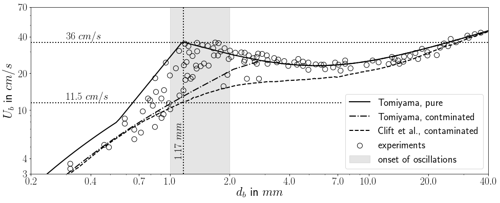
Rise velocity of air bubbles in water.
specimen calculation $d_b=1~mm$ pure water/oxygen at room temperature - kinematic viscosity water?
- $\nu_l\approx 10^{-3} m^2/s$
- $\nu_l\approx 10^{-4} m^2/s$
- $\nu_l\approx 10^{-5} m^2/s$
- $\nu_l\approx 10^{-6} m^2/s$
specimen calculation $d_b=1~mm$ pure water/oxygen at room temperature - molecular diffusivity oxygen in water?
- $D_{O_2}\approx 2\times 10^{-7} m^2/s$
- $D_{O_2}\approx 2\times 10^{-8} m^2/s$
- $D_{O_2}\approx 2\times 10^{-9} m^2/s$
- $D_{O_2}\approx 2\times 10^{-10} m^2/s$
Estimating the velocity boundary layer's thickness:
$$ Re = \frac{d_b U_b}{\nu_l} = \frac{0.25\times 10^{-3}}{10^{-6}} = 250 $$
$$ \frac{d_b}{\delta_h} \approx \sqrt{2Re} \approx 22 \rightarrow \delta_h\approx 45\mu m$$
Reference: A. Weiner 2019, p. 3, table 1.
Estimating the species boundary layer's thickness:
$$ Sc = \frac{\nu_l}{D_{O_2}} = \frac{10^{-6}}{2\times 10^{-9}} = 500 $$
$$ \frac{\delta_h}{\delta_c} \approx \frac{1}{\sqrt{Sc}} \sqrt{\pi/2} \approx 18 \rightarrow \delta_c\approx 2.5\mu m$$
Reference: A. Weiner et al. 2017, p. 3.
Summing up:
- $Pe = Sc\ Re = \nu_l / D_{O_2} \cdot U_b d_b/\nu_l \approx 10^5 $
- $$ Re\approx 250;\quad \delta_h/d_b \propto Re^{-1/2};\quad\delta_h\approx 45~\mu m $$
- $$ Sc\approx 500;\quad \delta_c/\delta_h \propto Sc^{-1/2};\quad\delta_c\approx 2.5~\mu m $$
$\delta_h/\delta_c$ typically 10 ... 100
feasible simulations up to $Pe\approx 1000$ (3D, HPC)
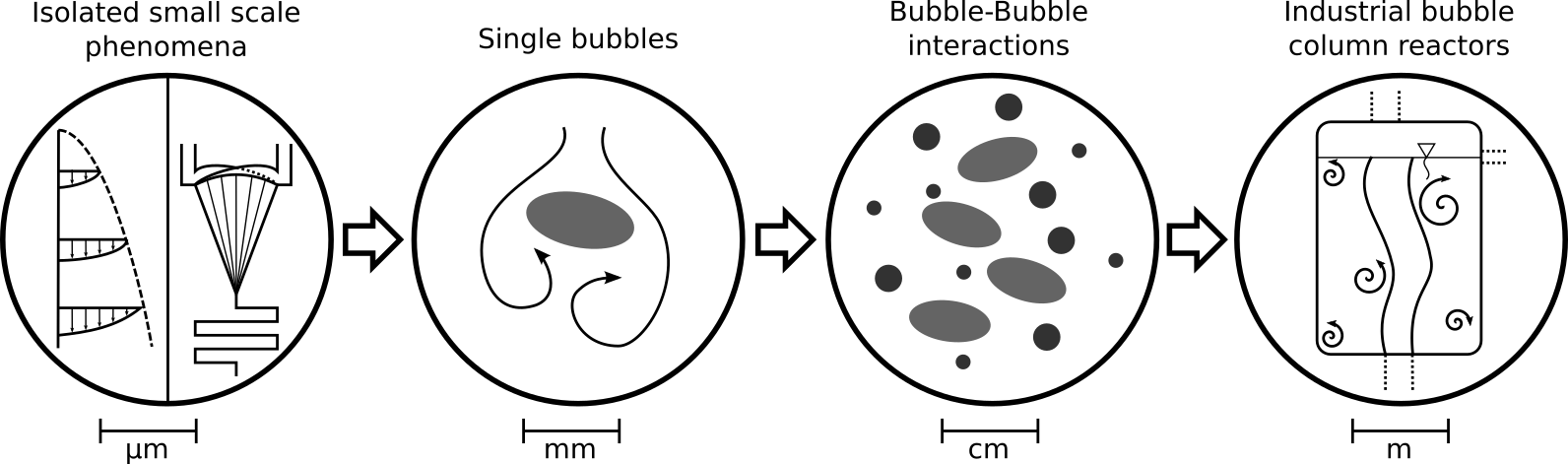
The bigger picture: scale-up strategy.
How can we approximate the species boundary layer with reasonable computational effort?
Solution: decoupling of two-phase flow problem and species transport.
Decoupling two-phase flow and species transport
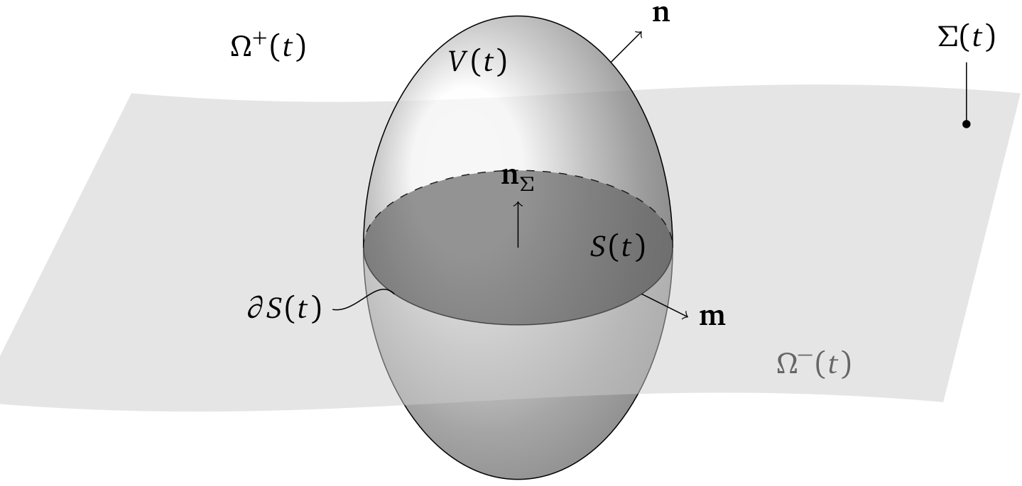
Sharp interface model: $t$ - time, $\Omega^+$ - liquid domain, $\Omega^-$ - gas domain, $\Sigma$ - interface, $V$ - control volume, $S$ - control surface, $\mathbf{n}_\Sigma$ - unit vector normal to $\Sigma$, $\partial S$ - boundary of $S$, $\mathbf{m}$ - unit vector normal to $\partial S$
Mass conservation:
$$ \frac{\partial \rho}{\partial t} + \nabla \cdot \left( \rho\mathbf{u} \right) = 0 $$
in $\Omega^\pm (t)$ - two equations!
Conservation of momentum:
$ \begin{align} \frac{\partial \rho \mathbf{u}}{\partial t} + \nabla \cdot \left( \rho \mathbf{u} \otimes \mathbf{u} \right) &=\\ &-\nabla p\\ &+ \nabla \cdot \left( \eta \left( \nabla \mathbf{u} + \nabla\mathbf{u}^\mathsf{T} \right) \right)\\ &+ \rho\mathbf{b} \end{align} $
in $\Omega^\pm (t)$ - two equations!
What happens at the interface? Definition of jump brackets for a generic variable $\varphi$:
$$ [\![ \varphi (t,\mathbf{x}) ]\!] = \lim_{h\to+0}\left(\varphi^+ (t,\mathbf{x} + h\mathbf{n}_\Sigma) - \varphi^- (t,\mathbf{x} - h\mathbf{n}_\Sigma)\right) $$
for $\mathbf{x}\in \Sigma (t)$
mass jump condition:
$$ \dot{m}^+ - \dot{m}^- = 0\quad \text{on}\quad \Sigma (t) $$
$$ \left[ \rho^+ \left( \mathbf{u}^+ - \mathbf{u}^\Sigma \right) - \rho^- \left( \mathbf{u}^- - \mathbf{u}^\Sigma \right)\right] \cdot \mathbf{n}_\Sigma = 0\quad \text{on}\quad \Sigma (t) $$
$$ [\![ \rho \left( \mathbf{u} - \mathbf{u}^\Sigma \right) ]\!] \cdot \mathbf{n}_\Sigma = 0\quad \text{on}\quad \Sigma (t) $$
$\mathbf{u}^\Sigma$ - interface velocity
neglecting mass transfer:
$$ \dot{m}^+ = \dot{m}^- = 0\quad \text{on}\quad \Sigma (t) $$
$\mathbf{u}^+\cdot \mathbf{n}_\Sigma = \mathbf{u}^\Sigma\cdot \mathbf{n}_\Sigma$ and $\mathbf{u}^-\cdot \mathbf{n}_\Sigma = \mathbf{u}^\Sigma\cdot \mathbf{n}_\Sigma$
typical assumption for tangential velocity component (not a consequence of mass conservation):
$$ [\![ \mathbf{u} ]\!] \cdot \mathbf{t}_\Sigma = 0 $$
$$\mathbf{u}^+\cdot \mathbf{t}_\Sigma = \mathbf{u}^-\cdot \mathbf{t}_\Sigma$$
$\mathbf{t}_\Sigma$ - unit vector tangential to interface
momentum jump conditions ...
Closest numerical approach to sharp interface model: interface tracking
Advantages and disadvantages of interface tracking:
- possibility to combine physical phenomena
- interface-aligned meshes
- very good accuracy at the interface
- extremely high complexity
- very slow
- stability issues
A one-field approach to two-phase flow simulations: the volume of fluid method
Advantages and disadvantages of volume of fluid solvers:
- Computationally efficient and robust
- Relatively easy to implement
- fields are phase-averaged
- bad accuracy close to the interface
Idea
combine computational efficiency of volume of fluid and the accuracy of surface-aligned meshes
1. Two-phase flow simulation (Volume-of-Fluid)
2. Single-phase flow solution
3. Species transport
Problem
Missing boundary conditions for
- velocity at the interface
- shape/mesh deformation
- rise/inlet velocity
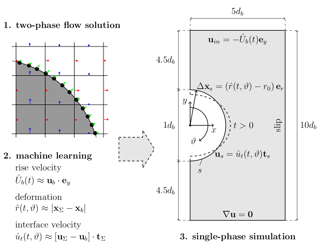
Creating models for deformation and velocity
Inlet boundary condition - first model:
$$ \mathbf{u}_{in} = -\tilde{U}_b\mathbf{e}_y $$
$\tilde{U}_b$ - the bubble's terminal velocity
What would be a more suitable ansatz for $\tilde{U}_b$?
- $\tilde{U}_b = f_\vartheta(\tilde{t})$
- $\tilde{U}_b = f_\vartheta(\tilde{t})\tilde{t}$
$f_\vartheta(\tilde{t})$ is a neural network model.
Which normalization is suitable for $\tilde{t}$?
- Min-Max, $\tilde{t}\in [-1, 1]$
- Min-Max, $\tilde{t}\in [0, 1]$
- Mean-Std.
Rise velocity model - normalized features and labels.
class RVModelNorm(pt.nn.Module):
    def __init__(self, n_neurons=100, n_hidden=2, activation=pt.nn.Tanh):
        super(RVModelNorm, self).__init__()
        self._model = create_simple_network(1, 1, n_neurons, n_hidden, activation)

    def forward(self, x):
        return self._model(x) * x

MSE loss for the normalized rise velocity.
Rise velocity model - final model
class RVModel(pt.nn.Module):
    def __init__(self, rv_model_norm, rv_min, rm_max, t_min, t_max):
        super(RVModel, self).__init__()
        self._model = rv_model_norm
        self._rv_min = rv_min
        self._rv_max = rv_max
        self._t_min = t_min
        self._t_max = t_max

    def forward(self, x):
        x_norm = (x.unsqueeze(1) - self._t_min) / (self._t_max - self._t_min)
        rv_norm = self._model(x_norm)
        return (rv_norm * (self._rv_max - self._rv_min) + self._rv_min).squeeze()

Comparison of model prediction and reference data for the rise velocity.
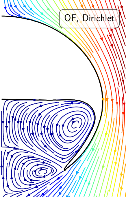
Interface velocity boundary condition - second model:
$$ \mathbf{u}_s = \tilde{u}_t\mathbf{t} $$
$$ \tilde{u}_t = \tilde{u}_t(\vartheta, \tilde{t}) $$
$\tilde{u}_t$ - tangential component of interface velocity vector.
What applies to the tangential interface velocity?
- line symmetry rise axis
- point symmetry $\vartheta = 0$, $\vartheta = \pi$
- no symmetry

Sine and cosine functions with vertical lines at $0$ and $\pi$.
How can we enforce the correct symmetry in the model?
- $\tilde{u}_t = f_\vartheta (\vartheta, \tilde{t})\mathrm{sin}(\vartheta)$
- $\tilde{u}_t = f_\vartheta (\vartheta, \tilde{t})\mathrm{cos}(\vartheta)$
- $\tilde{u}_t = f_\vartheta (\mathrm{sin}(\vartheta), \tilde{t})\mathrm{sin}(\vartheta)$
- $\tilde{u}_t = f_\vartheta (\mathrm{cos}(\vartheta), \tilde{t})\mathrm{sin}(\vartheta)$
Model for the normalized tangential velocity component.
class TVVelocityNorm(pt.nn.Module):
    def __init__(self, n_neurons=100, n_hidden=5, activation=pt.nn.ReLU):
        super(TVVelocityNorm, self).__init__()
        self._model_norm = create_simple_network(2, 1, n_neurons, n_hidden, activation)

    def forward(self, x):
        sin = pt.sin(x[:, 0]).unsqueeze(-1)
        x = pt.stack((pt.cos(x[:, 0]), x[:, 1])).T
        return self._model_norm(x) * sin * x[:, 1].unsqueeze(-1)

Training and validation loss for the normalized tangential velocity component.

Comparison of model prediction and reference data.
Interface deformation - third model:
$$ \Delta \mathbf{x} = (\tilde{r} - r_0)\mathbf{e}_r $$
$$ \tilde{r} = \tilde{r}(\vartheta, \tilde{t}) $$
What applies to the radius?
- line symmetry rise axis
- point symmetry $\vartheta = 0$, $\vartheta = \pi$
- no symmetry
Model for normalized bubble radius.
class RadNorm(pt.nn.Module):
    def __init__(self, n_neurons=100, n_hidden=5, activation=pt.nn.ReLU):
        super(RadNorm, self).__init__()
        self._model_norm = create_simple_network(2, 1, n_neurons, n_hidden, activation)

    def forward(self, x):
        x = pt.stack((pt.cos(x[:, 0]), x[:, 1])).T
        return self._model_norm(x) * x[:, 1].unsqueeze(-1)

Training and validation loss for the normalized radius.

Comparison of model prediction and reference data for the bubble radius.
Tracing and saving the final models
with pt.no_grad():
    rv_trace = pt.jit.trace(rv_model.eval(), example_inputs=pt.rand(2))
rv_trace.save(join(output, "rv_model.pt"))
Analyzing the results
Results for four different $Eo$ numbers; $Sc=100$.
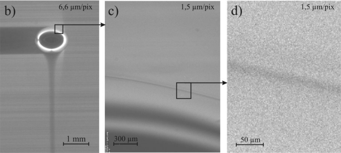
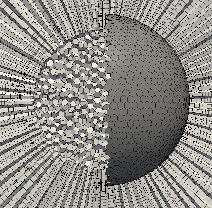
Mesh deformation and boundary layer zoom view.
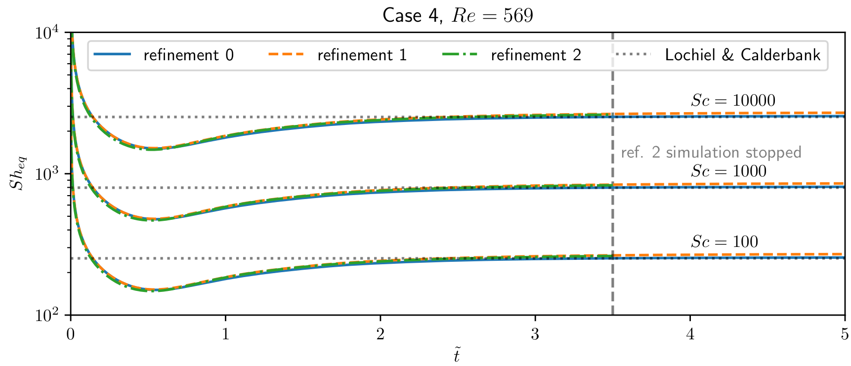
Dimensionless global mass transfer - Sherwood number $Sh$.
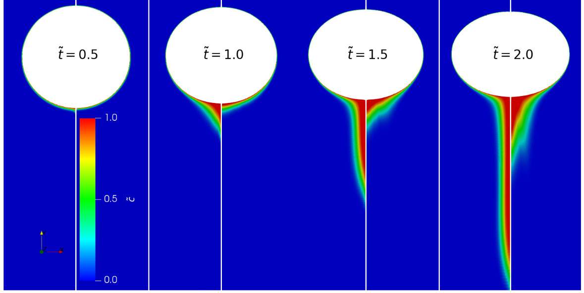
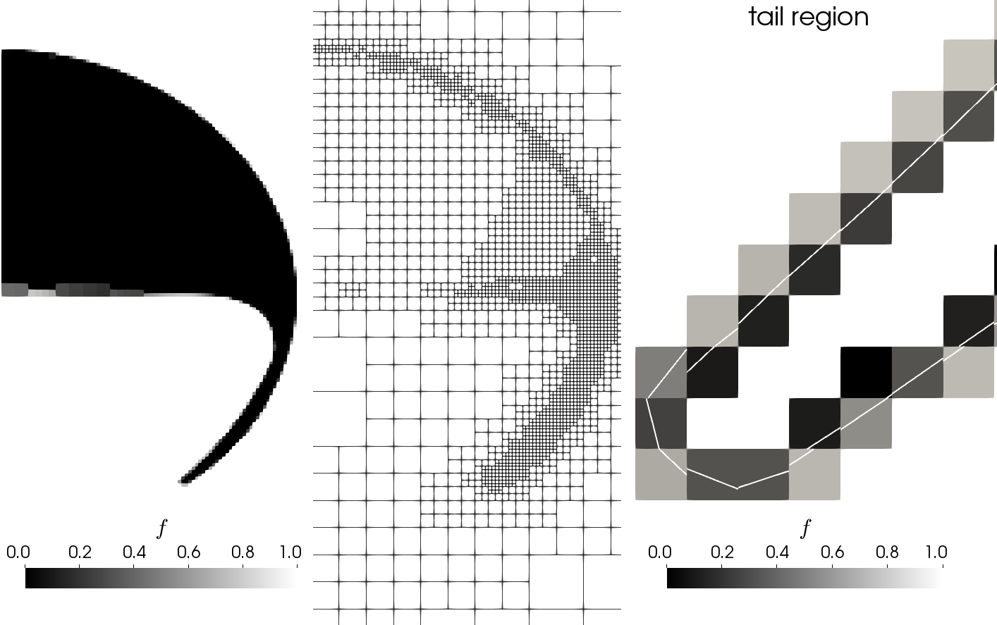
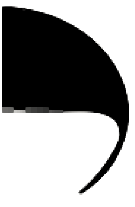
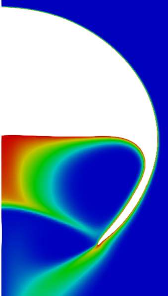
Wake concentration - slip vs. ML.
For more details refer to
Assessment of a subgrid-scale model for convection-dominated mass transfer for initial transient rise of a bubble