Reduced-order modeling for flow fields
Andre Weiner
TU Dresden, Institute of fluid mechanics, PSM

These slides and most
of the linked resources are licensed under a
Creative Commons Attribution 4.0
International License.
Last lecture(s)
Analyzing coherent structures in flows displaying transonic shock buffets
- transonic shock buffet
- principal component analysis (PCA)
- ways to compute the PCA
- dynamic mode decomposition (DMD)
Outline
Reduced-order modeling of flow fields
- reduced-order models for dynamical systems
- optimized DMD
- dealing with high-dimensional data
Reduced-order models for dynamical systems
What is a reduced-order model (ROM)?
- mathematical model with reduced
- computational complexity
- dimensionality
- approximation
- often derived from data
ROMs for dynamical systems
$$ \frac{\mathrm{d}\mathbf{x}}{\mathrm{d}t} = F(\mathbf{x}(t), t, ...) $$
Definition of ROMs in this lecture:
- encoding: $\tilde{\mathbf{x}}_n = E(\mathbf{x}_n)$
- evolution: $\tilde{\mathbf{x}}_{n+1} \approx f(\tilde{\mathbf{x}}_n)$
- decoding: $\hat{\mathbf{x}}_n \approx E^{-1}(\tilde{\mathbf{x}}_n)$
$\mathbf{x}$ - full state, $\tilde{\mathbf{x}}$ - reduced state, $\hat{\mathbf{x}}$ - full state prediction
Data-driven ROMs:
ML for encoding/decoding and/or temporal evolution.
Criteria for good ROMs:
- computationally efficient
- interpretable states and dynamics
- long-term stability
Optimized DMD
review of some DMD basics
- $\mathbf{x}_n$: state vector at time $t_n = n\Delta t$
- core idea: $ \mathbf{x}_{n+1}=\mathbf{A}\mathbf{x}_n $
- diagonalization: $\mathbf{A}=\mathbf{\Phi}\mathbf{\Lambda}\mathbf{\Phi}^{-1}$
- prediction: $\mathbf{x}_{n} = \mathbf{\Phi\Lambda}^{n-1}\mathbf{\Phi}^{-1}\mathbf{x}_1$
$\rightarrow$ once $\mathbf{A}$ is known, the state at any $t_n$ may be predicted based on a given initial state $\mathbf{x}_1$
reconstruction of the full dataset
$$ \underbrace{ \begin{bmatrix} x_{11} & \ldots & x_{1N}\\ \vdots & \ddots & \vdots\\ x_{M1} & \ldots & x_{MN} \end{bmatrix} }_{\mathbf{M}} \approx \underbrace{ \begin{bmatrix} \phi_{11} & \ldots & \phi_{1r}\\ \vdots & \ddots & \vdots\\ \phi_{M1} & \ldots & \phi_{Mr} \end{bmatrix} }_{\mathbf{\Phi}} \underbrace{ \begin{bmatrix} b_1& & \\ & \ddots & \\ & & b_r \end{bmatrix} }_{\mathbf{D_b}} \underbrace{ \begin{bmatrix} \lambda_{1}^0 & \ldots & \lambda_{1}^{N-1}\\ \vdots & & \vdots\\ \lambda_r^0 & \ldots & \lambda_r^{N-1} \end{bmatrix} }_{\mathbf{V_\lambda}} $$
with $\mathbf{b} = \mathbf{\Phi}^{-1}\mathbf{x}_1$, $M$ - length of $\mathbf{x}$, $N$ - number of snapshots, $r$ - truncation rank
regular DMD
$\mathbf{X} = \left[ \mathbf{x}_1, \ldots, \mathbf{x}_{N-1} \right]^T$$\mathbf{Y} = \left[ \mathbf{x}_2, \ldots, \mathbf{x}_{N} \right]^T$
$$ \underset{\mathbf{A}}{\mathrm{argmin}}\left|\left| \mathbf{Y}-\mathbf{AX} \right|\right|_F $$
optimizedDMD
$\mathbf{\Phi_b}=\mathbf{\Phi}\mathbf{D_b}$$\mathbf{M} = \left[ \mathbf{x}_1, \ldots, \mathbf{x}_{N} \right]^T$
$$ \underset{\mathbf{\lambda},\mathbf{\Phi}_\mathbf{b}}{\mathrm{argmin}}\left|\left| \mathbf{M}-\mathbf{\Phi}_\mathbf{b}\mathbf{V}_{\mathbf{\lambda}} \right|\right|_F $$
$\rightarrow$ "optDMD" problem is non-linear and non-convex
idea: borrow techniques from ML/DL
- stochastic gradient descent
- automatic differentiation
- train-validation-split
- early stopping
$\rightarrow$ refer to article for details
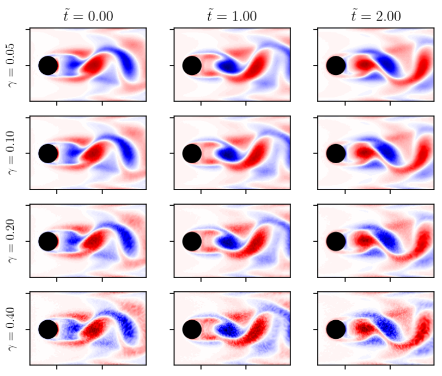
Test data with noise corruption.
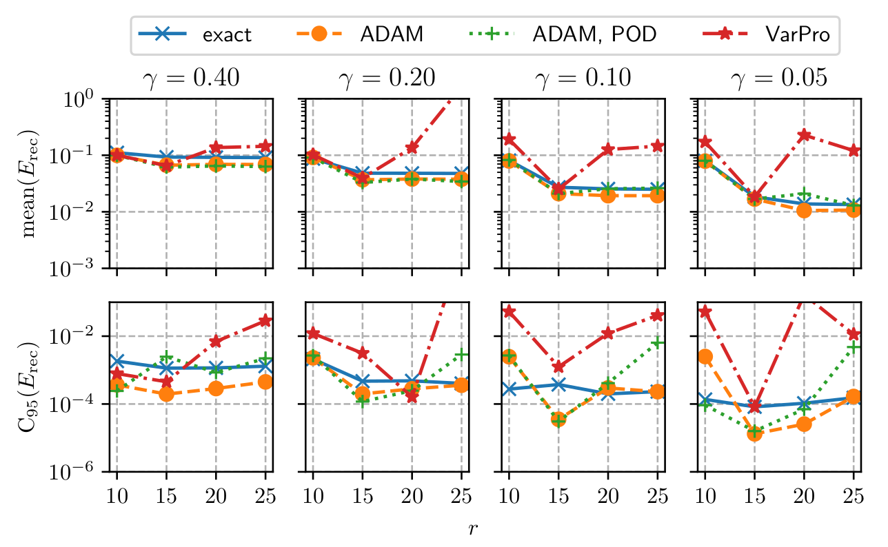
Comparison of DMD reconstruction error.
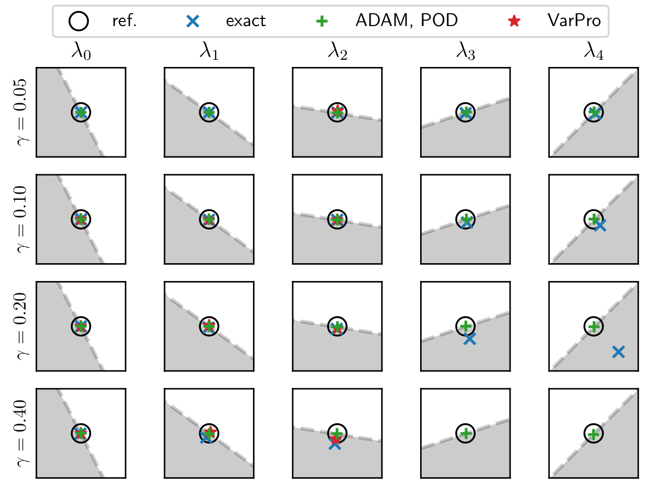
Comparison of dominant eigenvalues; reference computed with clean data.
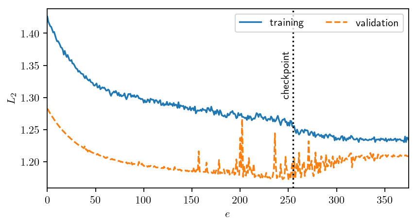
Early stopping prevents overfitting.
optimized DMD with sparsity promotion
$$ \underset{\mathbf{\lambda},\mathbf{\Phi}_\mathbf{b}}{\mathrm{argmin}}\left(\left|\left| \mathbf{M}-\mathbf{\Phi}_\mathbf{b}\mathbf{V}_{\mathbf{\lambda}} \right|\right|_F + \gamma_0 ||\mathbf{b}||_2\right) $$
$\rightarrow$ reduction to dominant dynamics
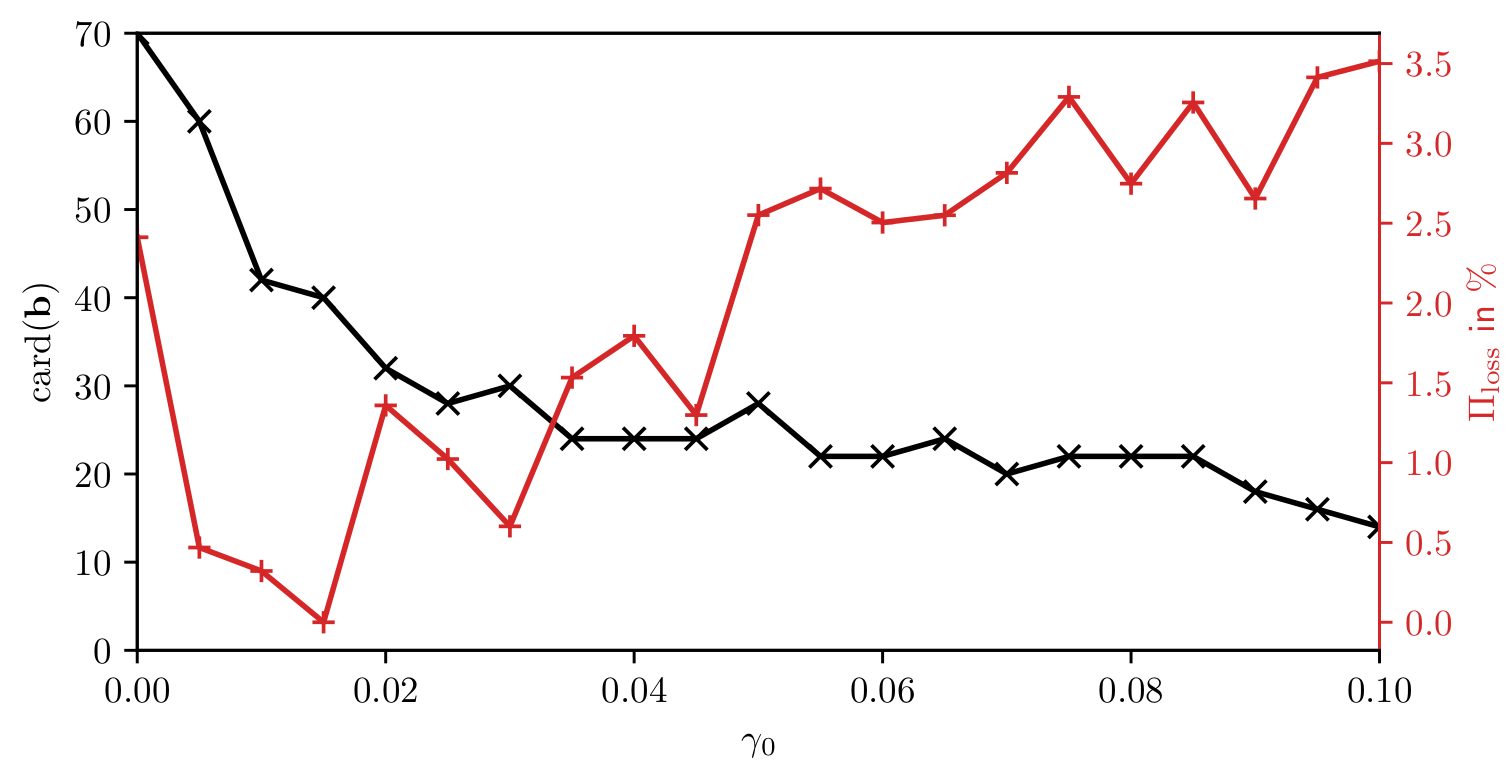
Cardinality of modes amplitudes and reconstruction error for increasing sparsity weight $\gamma_0$.
dealing with high-dimensional data
most common strategies
- project data on POD modes
- (variational) autoencoder
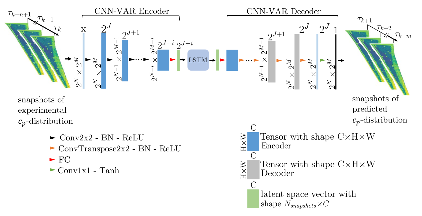
CNN-VAR-AE + LSTM; figure 2 from Zahn et al. (2023).
