Goals of flow control:

• drag reduction
• load reduction
• process intensification
• noise reduction
• ...

Categories of flow control:

1. passive: modification of geometry, topology, fluid, ...
2. active: flow actuation through moving parts, blowing/suction, heating/cooling, ...

Active flow control can be more effective but requires energy.

Categories of active flow control:

1. open-loop: actuation prescript; constant or periodic motion, blowing, heating, ...
2. closed-loop: actuation based on sensor input

Closed-loop flow control can be more effective but defining the control law is extremely challenging.

Flow past a circular cylinder at $Re=100$.

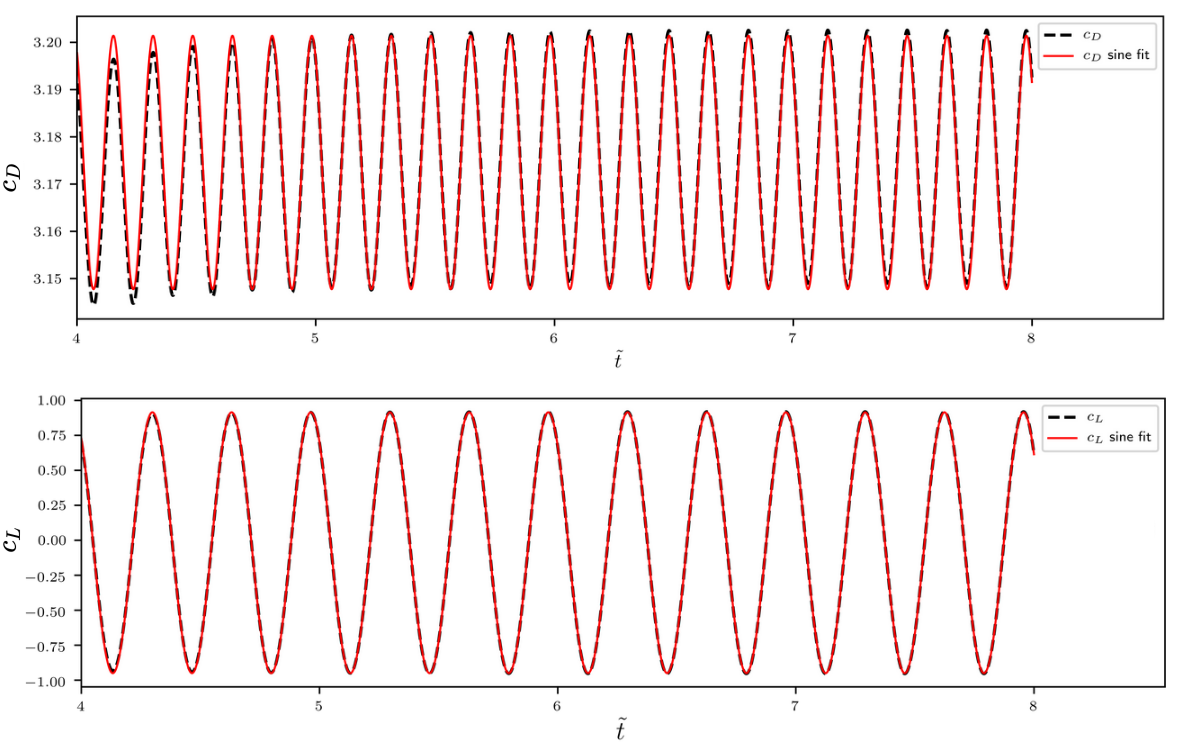
Drag and lift coefficients for the cylinder surface; source: figure 2.9 in D. Thummar 2021.

Typical steps in open-loop control:

1. define (parametrized) control law
2. optional: optimize control law
   • define loss/objective function
   • optimize control law iteratively

Open-loop example:

• periodic cylinder rotation with
  $$\omega = A \mathrm{sin}(2\pi ft)$$
• optimization of $A$ and $f$ by searching
• loss
  $$\Phi = \sqrt{\bar{C_D}^2 + \bar{C_L}^2 + (C_{D_{max}}-C_{D_{min}})^2 +(C_{L_{max}}-C_{L_{min}})^2}$$
• $\Omega = d/(2\bar{U}) A$ and $S_f = d/\bar{U}f$

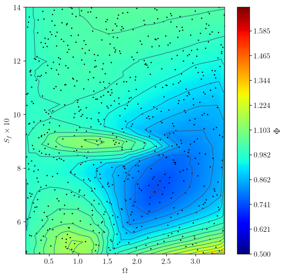
Loss landscape for periodic control; source: figure 3.5 in D. Thummar 2021.

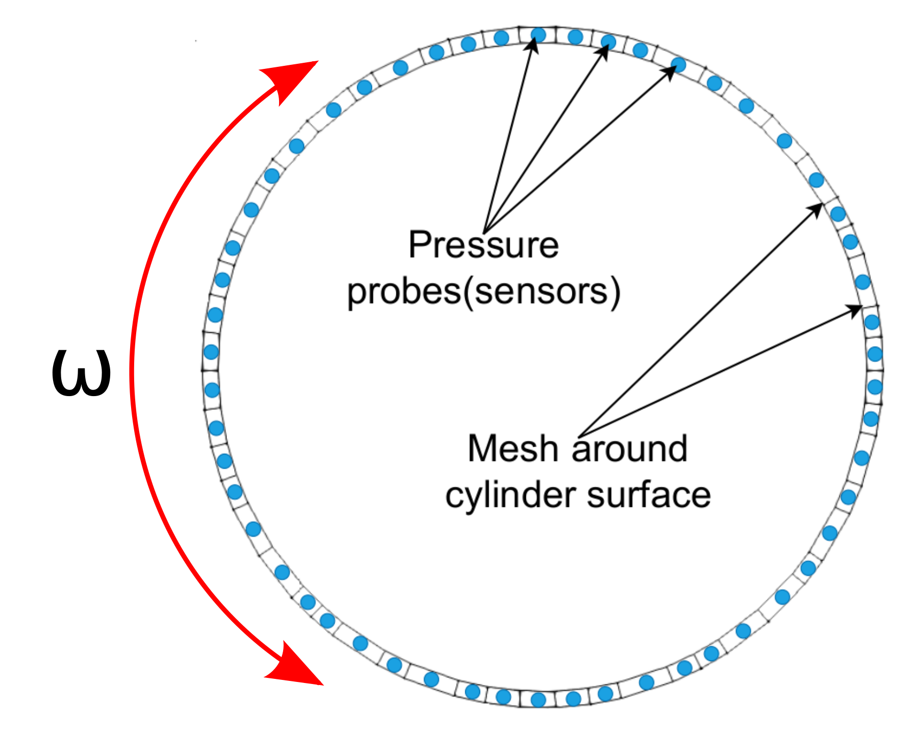
Closed-loop example: $\omega = f(\mathbf{p})$.

Closed-loop flow control with variable Reynolds number; source: F. Gabriel 2021.

How to find the control law?

• careful manual design
• Bayesian optimization
• machine learning control (MLC)
• (deep) reinforcement learning (DRL)

Favorable attributes of DRL:

• sample efficient thanks to NN-based function approximation
• discrete, continuous, or mixed states and actions
• control law is learnt from scratch
• can deal with uncertainty
• high degree of automation possible

Why CFD-based closed-loop control via DRL?

• save virtual environment
• prior optimization, e.g., sensor placement

Main challenge: CFD environments are expensive!

Reinforcement learning cycle.

The agent:

• interacts, evaluates, improves
• acts on the environment following a policy $\pi$
• observes how the state changes
• receives a reward from the environment
• evaluates and improves policy

The environment at time step $n$:

• is defined by a state $S_n$
• transitions from $S_n$ to $S_{n+1}$ when acted on
• returns a reward $R_n$
• defines an extrinsic task expressed by reward

State $S_n\in \mathcal{S}$:

• defines environment
• can be discrete, continuous, or mixed
• lies in the state space $\mathcal{S}$
• are typically not fully available $\rightarrow$ observation
• change upon action according to transition function

Note that state and observation are typically used as synonyms.

Action $A_n\in \mathcal{A}(s)$:

• is determined by policy $\pi (s)$
• lies in the action space $\mathcal{A}(s)$
• may be state-dependent
• can be discrete, continuous, or mixed

Even more definitions:

• task: overall goal; episodic or continuing
• time step $n$: one interaction between agent and environment
• episode: cumulation of time steps in episodic tasks
• horizon: time step limit; finite or infinite
• experience tuple: $\{ S_n, A_n, R_{n+1}, S_{n+1}\}$
• trajectory: all experience tuples in an episode

Describing uncertainty: "slippery walk" presented as Markov decision process (MDP).

Markov property:

$$P(S_{n+1}|S_n, A_n) = P(S_{n+1}|S_n, A_n, S_{n-1}, A_{n-1}, ...)$$

May be relaxed in practice by adding several time levels to the state.

Transition function:

$$p(s^\prime | s, a) = P(S_{n}=s^\prime | S_{n-1} = s, A_{n-1} = a)$$

Reward function:

$$r(s, a) = \mathbb{E}[R_{n} | S_{n-1}=s, A_{n-1}=a]$$

What are the upper and lower case letters about?

Slippery walk in gym/gym_walk:

env = gym.make('SlipperyWalkSeven-v0')
init_state = env.reset()
P = env.env.P
list(P.items())[-2:]
# output
[(7,
  {0: [(0.5000000000000001, 6, 0.0, False),
    (0.3333333333333333, 7, 0.0, False),
    (0.16666666666666666, 8, 1.0, True)],
   1: [(0.5000000000000001, 8, 1.0, True),
    (0.3333333333333333, 7, 0.0, False),
    (0.16666666666666666, 6, 0.0, False)]}),
 (8,
  {0: [(0.5000000000000001, 8, 0.0, True),
    (0.3333333333333333, 8, 0.0, True),
    (0.16666666666666666, 8, 0.0, True)],
   1: [(0.5000000000000001, 8, 0.0, True),
    (0.3333333333333333, 8, 0.0, True),
    (0.16666666666666666, 8, 0.0, True)]})]
						

• state space: $s\in \{0, 1, 2, 3, 4, 5, 6, 7, 8 \}$
• action space: $a \in \{0, 1\}$
• reward space: $r \in \{0, 1\}$
• experience tuple: $(3, 0, 0, 4)$
• trajectory: $((5, 0, 0, 6), (6, 1, 0, 7), ...)$

What is the meaning of $(3, 0, 0, 4)$?

1. action go right
2. transition from 4 to 3
3. reward of 0

Why might the CFD environment be uncertain?

1. random actions
2. random state changes
3. incomplete state (observation)

Intuitively, what is the optimal policy?

1. always go left
2. always go right
3. alternate left and right
4. depends on initial state
5. it doesn't matter - all policies optimal

Dealing with sequential feedback:

return: $$G_n = R_{n+1} + R_{n+2} + ... + R_N$$

discounted return: $$G_n = R_{n+1} + \gamma R_{n+2} + \gamma^2 R_{n+3} + ... \gamma^{N-1}R_N$$

$N$ - number of time steps, $\gamma$ - discounting factor, typically $\gamma = 0.99$

recursive definition: $$G_n = R_{n+1} + \gamma R_{n+2} + \gamma^2 R_{n+3} + ... \gamma^{N-1}R_N$$ $$G_{n+1} = R_{n+2} + \gamma R_{n+3} + \gamma^2 R_{n+4} + ... \gamma^{N-1}R_N$$ $$G_n = R_{n+1} + \gamma G_{n+1}$$

Why should we discount?

rewards trajectory 1: $(0, 0, 0, 0, 1)$
rewards trajectory 2: $(0, 0, 0, 0, 0, 0, 1)$

Which one is better?

returns: 1 and 1

discounted returns: $0.99^5\cdot 1$ and $0.99^7\cdot 1$

$\rightarrow$ discounting expresses urgency

Returns combined with uncertainty: the state-value function

$$v_\pi (s) = \mathbb{E}_\pi [G_n| S_n=s] = \mathbb{E}_\pi [R_{n+1} + \gamma G_{n+1}| S_n=s]$$ In words: the value function expresses the expected return at time step $n$ given that $S_n = s$ when following policy $\pi$.

How to compute the value-function if the MDP is known? - Bellman equation

$$v_\pi (s) = \mathbb{E}_\pi [R_{n+1} + \gamma G_{n+1}| S_n=s]$$ $$v_\pi (s) = \sum\limits_{s^\prime , r, a} p(s^\prime,r| s, a) [r + \gamma \mathbb{E}_\pi [G_{n+1} | S_{n+1} = s^\prime)]]$$ $$v_\pi (s) = \sum\limits_{s^\prime , r, a} p(s^\prime,r| s, a) [r + \gamma v_\pi (s^\prime)]\quad \forall s\in S$$

$s^\prime$ - next state; deterministic actions assumed

Intuitively, which state has the highest value?

1. 0
2. 3
3. 5
4. 6
5. all equal

What action to take? The state-action function:

$$q_\pi (s, a) = \mathbb{E}_\pi [G_n | S_n = s, A_n=a]$$ $$q_\pi (s, a) = \mathbb{E}_\pi [R_{n+1} + \gamma G_{n+1} | S_n = s, A_n=a]$$ $$q_\pi (s, a) = \sum\limits_{s^\prime , r} p(s^\prime,r| s, a)[r + \gamma v_\pi (s^\prime)]\quad \forall s\in S, \forall a\in A$$

Intuitively, what would you expect $q_\pi (s, a=0)$ vs. $q_\pi (s, a=1)$ ?

1. $q_\pi (s, a=0) > q_\pi (s, a=1)$
2. $q_\pi (s, a=0) = q_\pi (s, a=1)$
3. $q_\pi (s, a=0) < q_\pi (s, a=1)$

How much better is an action? - action-advantage function

$$a_\pi (s,a) = q_\pi(s,a) - v_\pi(s)$$

The optimal policy:

$$v^\ast (s) = \underset{\pi}{\mathrm{max}}\ v_\pi (s)\quad \forall s\in \mathcal{S}$$ $$q^\ast (s, a) = \underset{\pi}{\mathrm{max}}\ q_\pi (s, a)\quad \forall s\in \mathcal{S}, \forall a\in \mathcal{A}$$

Planning: finding $\pi^\ast$ with value iterations

$$v_{k+1}(s) = \underset{a}{\mathrm{max}}\sum\limits_{s^\prime, r} p(s^\prime , r | s, a)[r+\gamma v_k(s^\prime)]$$

$v_k$ - value estimate at iteration $k$

Value iteration implementation:

def value_iteration(P: Dict[int, Dict[int, tuple]], gamma: float=0.99, theta: float=1e-10):
    V = pt.zeros(len(P))
    while True:
        Q = pt.zeros((len(P), len(P[0])))
        for s in range(len(P)):
            for a in range(len(P[s])):
                for prob, next_state, reward, done in P[s][a]:
                    Q[s][a] += prob * (reward + gamma * V[next_state] * (not done))
        if pt.max(pt.abs(V - pt.max(Q, dim=1).values)) < theta:
            break
        V = pt.max(Q, dim=1).values
    pi = lambda s: {s:a for s, a in enumerate(pt.argmax(Q, dim=1))}[s]
    return Q, V, pi
						

Optimal action-value function:

optimal_Q, optimal_V, optimal_pi = value_iteration(P)
optimal_Q[1:-1]
# output
tensor([[0.3704, 0.6668],
        [0.7902, 0.8890],
        [0.9302, 0.9631],
        [0.9768, 0.9878],
        [0.9924, 0.9960],
        [0.9976, 0.9988],
        [0.9993, 0.9997]])
						

Why is it called reinforcement learning and not planning?

1. both are equivalent
2. reward function unknown
3. transition function unknown
4. reward and transition function unknown

Deep RL uses neural networks to learn function approximations of:

• the action-value function
• the value function
• the policy
• the environment
• combinations of all points above

Some DRL lingo:

• Value-based methods: approximation of action-value function; NFQ, DQN, DDQN
• Policy-gradient methods: approximation of policy; REINFORCE, VPG
• Model-based methods: approximation of environment; PILCO, METRPO
• Actor-critic methods: approximation of policy and value function with bootstrapping; A2C, PPO

General learning strategy:

1. initialize random policy/action-value functions
2. sample trajectory/trajectories from one or more environments
3. update network(s)
4. go back to 2. until convergence

How do DRL agents explore?

• discrete actions: equivalent to tabular methods
• continuous actions:
  • add noise to action
  • sample action from PDF

PDF - probability density function

Closed-loop example: $\omega = f(\mathbf{p})$.

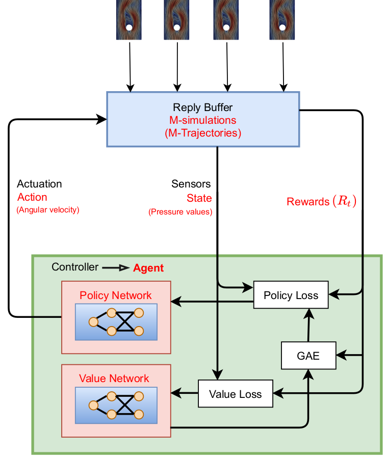
PPO overview; source: figure 4.6 in D. Thummar 2021.

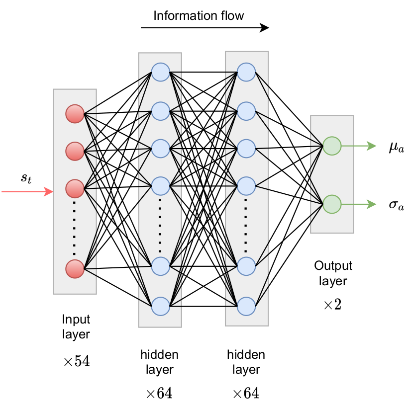
Policy network; source: figure 4.4 in D. Thummar 2021.

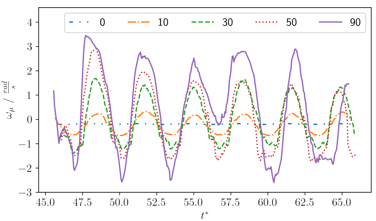
Action of example trajectories in training mode; source: figure 5.2 in F. Gabriel 2021.

Comparison of Gauss and Beta distribution.

learning what to expect in a given state - value function loss

$$L_V = \frac{1}{N_\tau N} \sum\limits_{\tau = 1}^{N_\tau}\sum\limits_{n = 1}^{N} \left( V(s_n^\tau) - G_n^\tau \right)^2$$

• $\tau$ - trajectory (single simulation)
• $s_n$ - state/observation (pressure)
• $V$ - parametrized value function
• clipping not included

Was the selected action a good one?

$$\delta_n = R_n + \gamma V(s_{n+1}) - V(s_n)$$ $$\delta_{n+1} = R_n + \gamma R_{n+1} + \gamma^2 V(s_{n+2}) - V(s_n)$$ $$A_n^{GAE} = \sum\limits_{l=0}^{N-n} (\gamma \lambda)^l \delta_{n+l}$$

• $\delta_n$ - one-step advantage estimate
• $A_n^{GAE}$ - generalized advantage estimate
• $\lambda$ - smoothing parameter

make good actions more likely - policy objective function

$$J_\pi = \frac{1}{N_\tau N} \sum\limits_{\tau = 1}^{N_\tau}\sum\limits_{n = 1}^{N} \mathrm{min}\left[ \frac{\pi(a_n|s_n)}{\pi^{old}(a_n|s_n)} A^{GAE,\tau}_n, \mathrm{clamp}\left(\frac{\pi(a_n|s_n)}{\pi^{old}(a_n|s_n)}, 1-\epsilon, 1+\epsilon\right) A^{GAE,\tau}_n\right]$$

• $\pi$ - current policy
• $\pi^{old}$ - old policy (previous episode)
• entropy not included
• $J_\pi$ is maximized

Effect of clipping in the PPO policy loss function.

Why PPO?

• continuous and discrete actions spaces
• relatively simple implementation
• restricted (robust) policy updates
• sample efficient
• ...

Refer to R. Paris et al. 2021 and the references therein for similar works employing PPO.

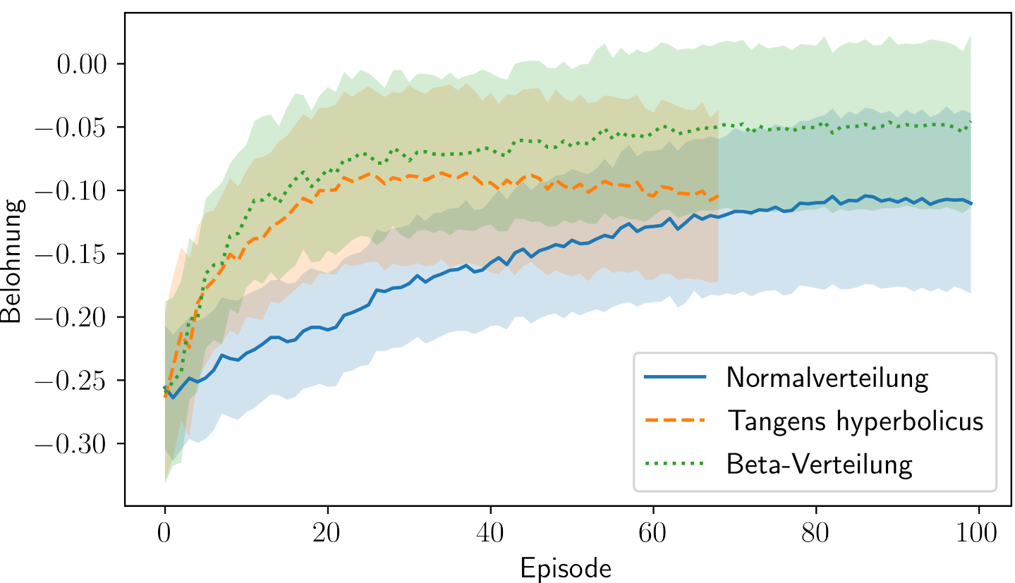
Cumulative reward over the number of training episodes; source: figure 5.8 in F. Gabriel 2021.

Closed-loop flow control with variable Reynolds number; source: F. Gabriel 2021.

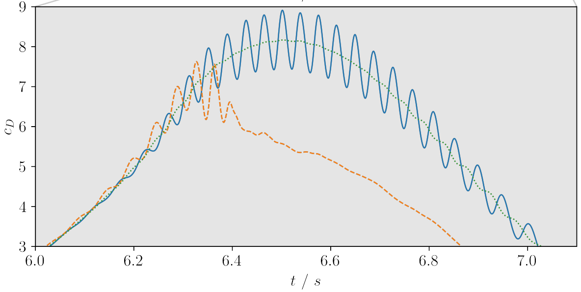
Drag coefficient with and without control; source: figure 6.5 in F. Gabriel 2021.

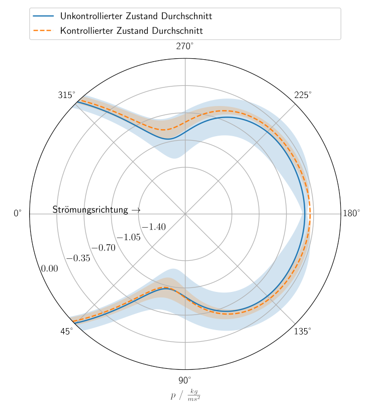
Pressure on the cylinder's surface; source: figure 5.7 in F. Gabriel 2021.