Transonic shock buffets

Boeing 737 undergoing buffet/stall - source.

Slice of local Mach number $Ma=0.75$, 3D, $\alpha=4^\circ$.

• self-sustained shock-BL-interactions
• may lead to aeroelastic reaction (buffeting)
• potentially influenced by acoustic waves
• very different for profiles (2D) and wings (3D)

Understanding shock buffet enables:

1. prediction of onset ($Ma$-$\alpha$ envelop)
2. passive or active control strategies

Principal component analysis (PCA)

Flow past a circular cylinder at $Re=100$.

Temporal mean and variance of velocity components.

Probe locations for velocity fluctuations.

Streamwise velocity fluctuations over time.

$u^\prime_1$ plotted against $u^\prime_2$.

Let's organize the data in a matrix:

$$ \mathbf{X} = \left[ \begin{array}{cccc} | & | & & | \\ \mathbf{u}^\prime_1 & \mathbf{u}^\prime_2 & ... & \mathbf{u}^\prime_{N} \\ | & | & & | \\ \end{array}\right] $$

$\mathbf{X}$ has as many rows as we have samples and as many columns as we have snapshots.

Projecting all the points ($u^\prime_1$-$u^\prime_2$-pairs) onto a vector:

$$ \mathbf{y} = \mathbf{\phi}^T \mathbf{X} $$

Our vector $\mathbf{\phi}$ has two rows and one column.

Effect of projection onto $\mathbf{\phi} = (1, -1)^T/\sqrt{2}$.

Computing the variance along $\mathbf{\phi}$:

$$ \mathrm{var}(\mathbf{y}) = \mathbf{yy}^T = \mathbf{\phi}^T \mathbf{X} (\mathbf{\phi}^T \mathbf{X})^T = \mathbf{\phi}^T \mathbf{XX}^T \mathbf{\phi} $$

Definition of the covariance matrix $\mathbf{C}$:

$$ \mathbf{C} = \frac{1}{N-1} \mathbf{XX}^T. $$

Covariance matrix in the natural basis.

Data projected onto rotated coordinate systems.

Covariance matrix in rotated coordinate systems.

PCA idea: find new orthogonal basis such that variance along each axis is maximized.

$\mathbf{C} = \mathbf{\Phi \Lambda \Phi}^{-1}\quad\text{given that}\quad \mathbf{\phi}^T_i\mathbf{\phi}_i = 1$

(proof in lecture notebook)

Principal components (optimal basis).

Mode coefficients $\mathbf{A}$:

$$ \mathbf{A} = \mathbf{\Phi}^T \mathbf{X} $$

Applied to snapshots, the coefficients encode the importance of each mode over time.

Mode coefficients probe data.

What if we take all points instead of two samples?

Mode coefficients probe data.

Modal decomposition: decomposition of snapshot data into modes (vary in space, const. in time) and temporal behavior (mode coefficients).

Ways to compute the PCA

Preliminaries - singular value decomposition (SVD):

$$ \mathbf{X} = \mathbf{U\Sigma V}^T $$

• $\mathbf{U}$ - left singular vectors
• $\mathbf{\Sigma}$ - singular values
• $\mathbf{V}$ - right singular vectors
• $\mathbf{U}$ and $\mathbf{V}$ are orthonormal
• non-zero $\sigma_{ij}$ on diagonal of $\mathbf{\Sigma}$

What applies to an orthonormal matrix?

1. $\mathbf{UU}^T = \mathbf{I}$
2. $\mathbf{U}^T \mathbf{U} = \mathbf{I}$
3. $\mathbf{U}^T = \mathbf{U}^{-1}$
4. all of the above

Economy SVD:

• $\mathbf{U}\in \mathbf{R}^{M\times N}$
• $\mathbf{\Sigma}\in \mathbf{R}^{N\times N}$
• $\mathbf{V}\in \mathbf{R}^{N\times N}$
• $\mathbf{U}^T\mathbf{U}=\mathbf{I}$, but $\mathbf{U}\mathbf{U}^T\neq\mathbf{I}$

Preliminaries - matrix inversion by SVD:

$$ \mathbf{X} = \mathbf{U\Sigma V}^T $$

$$ \mathbf{X}^{-1} = (\mathbf{U\Sigma V}^T)^{-1} = \mathbf{V}(\mathbf{U\Sigma})^{-1} = \mathbf{V}\mathbf{\Sigma}^{-1}\mathbf{U}^T $$

Data and covariance matrix:

$$ \mathbf{X} = \left[ \begin{array}{cccc} | & | & & | \\ \mathbf{x}_1 & \mathbf{x}_2 & ... & \mathbf{x}_{N} \\ | & | & & | \\ \end{array}\right] $$

$$ \mathbf{C} = \frac{1}{N-1} \mathbf{XX}^T $$

$\mathbf{x}_i$ - $i$th snapshot, $N$ - number of snapshots

Direct PCA:

$$ \mathbf{C} = \mathbf{\Phi \Lambda \Phi}^{T} $$

• $\mathbf{\Phi} \in \mathbb{R}^{M\times M}$ ($M$ - number of spatial points)
• $\mathbf{\Lambda} \in \mathbb{R}^{M\times M}$, diagonal
• column vectors $\mathbf{\phi}_j$ are called principal component or proper orthogonal decomposition (POD) modes
• $\mathbf{\Phi}$ is orthonormal, $\mathbf{\phi}_j$ form an orthonormal basis
• eigenvalues $\lambda_j$ are the variance along $\mathbf{\phi}_j$

Mode coefficients:

$$ \mathbf{A} = \mathbf{\Phi}^T \mathbf{X} \rightarrow \mathbf{X} = \mathbf{\Phi A} $$

• $\mathbf{A}$ - mode coefficient matrix
• $\mathbf{x}_i = \sum\limits_{j=1}^N a_{ji} \mathbf{\phi}_j$
• temporal behavior in row vectors of $\mathbf{A}$

Connection between direct PCA and SVD:

$$ \mathbf{C} = \frac{1}{N-1}\mathbf{XX}^T = \frac{1}{N-1} \mathbf{U\Sigma V}^T\mathbf{V\Sigma}^T\mathbf{U}^T = \frac{1}{N-1} \mathbf{U\Sigma}^2\mathbf{U}^T = \mathbf{\Phi\Lambda\Phi}^T $$

• $\mathbf{U}=\mathbf{\Phi}$
• $\mathbf{\Lambda} = \frac{\mathbf{\Sigma}^2}{N-1}$ (not for economy SVD)
• $\mathbf{A}=\mathbf{\Phi}^T \mathbf{X} = \mathbf{U}^T\mathbf{U\Sigma V}^T = \mathbf{\Sigma V}^T$

Snapshot PCA:

$$ \mathbf{C}_s = \frac{1}{N-1} \mathbf{X}^T\mathbf{X} = \mathbf{\Phi}_s\mathbf{\Lambda}_s\mathbf{\Phi}_s^T $$ $$ \mathbf{C}_s = \frac{1}{N-1} \mathbf{V\Sigma}^T\mathbf{U}^T\mathbf{U\Sigma V}^T = \frac{1}{N-1} \mathbf{V\Sigma}^2\mathbf{V}^T $$

• $\mathbf{C}$ and $\mathbf{C}_s$ have the same non-zero eigenvalues
• $\mathbf{\Phi}_s = \mathbf{V}$

Snapshot PCA - modes and coefficients:

$$ \mathbf{\Sigma} = \sqrt{\mathbf{\Lambda}_s (N-1)} $$

$$ \mathbf{A} = \mathbf{\Sigma} \mathbf{V}^T = (\mathbf{\Lambda}_s (N-1))^{1/2} \mathbf{\Phi}_s $$

$$ \mathbf{X\Phi}_s = \mathbf{U\Sigma V}^T\mathbf{\Phi}_s = \mathbf{U\Sigma V}^T\mathbf{V} = \mathbf{U\Sigma} $$ $$ \mathbf{\Phi} = \mathbf{U} = \mathbf{X\Phi}_s\mathbf{\Sigma}^{-1} = \mathbf{X\Phi}_s (\mathbf{\Lambda}_s(N-1))^{-1/2} $$

assumption: economy SVD

More variants available specialized for:

• distributed parallel systems
• large datasets
• datasets with noise
• streaming datasets

Dynamic mode decomposition (DMD)

Core idea:

$$ \mathbf{x}_{n+1} = \mathbf{Ax}_n $$

• $\mathbf{x}\in \mathbb{R}^M$ - state vector
• $\mathbf{A}\in \mathbb{R}^{M\times M}$ - linear operator

How to approximate $\mathbf{A}$?

$$ \underbrace{[\mathbf{x}_2, ..., \mathbf{x}_N]}_{\mathbf{Y}} = A \underbrace{[\mathbf{x}_1, ..., \mathbf{x}_{N-1}]}_{\mathbf{X}} $$

$$ \underset{\mathbf{A}}{\mathrm{argmin}} ||\mathbf{Y}-\mathbf{AX}||_F = \mathbf{YX}^\dagger $$

best-fit (least squares) linear operator

Probe locations for velocity fluctuations.

Computing $\mathbf{A}$ in PyTorch:

X = pt.stack((Up_p1, Up_p2))
U, s, VT = pt.linalg.svd(X[:, :-1], full_matrices=False)
A = X[:, 1:] @ VT.T @ pt.diag(1/s) @ U.T
A
# output
tensor([[ 0.4526, -0.4412],
        [ 0.0749,  0.9579]])
# testing the operator
Xpred = A @ X[:, :-1]
						

Probe locations for velocity fluctuations.

Can we predict the time series using only $\mathbf{x}_1$?

$$ \mathbf{x}_2 = \mathbf{Ax}_1 $$ $$ \mathbf{x}_3 = \mathbf{Ax}_2 = \mathbf{AAx}_1 = \mathbf{A}^2\mathbf{x}_1 $$ $$ \mathbf{x}_n = \mathbf{A}^{n-1}\mathbf{x}_1 $$

Step-by-step prediction:

Xpred[:, 0] = A @ X[:, 0]
for n in range(1, X.shape[1]-1):
    Xpred[:, n] = A @ Xpred[:, n-1]
						

Probe locations for velocity fluctuations.

What happened?

The eigen decomp. of $\mathbf{A}$ can help:

$$ \mathbf{A} = \mathbf{\Phi\Lambda\Phi}^{-1} $$ $$ \mathbf{x}_2 = \mathbf{Ax}_1 = \mathbf{\Phi\Lambda\Phi}^{-1} \mathbf{x}_1 $$ $$ \mathbf{x}_3 = \mathbf{AAx}_1 = \mathbf{\Phi\Lambda\Phi}^{-1}\mathbf{\Phi\Lambda\Phi}^{-1} \mathbf{x}_1 = \mathbf{\Phi\Lambda}^{2}\mathbf{\Phi}^{-1} \mathbf{x}_1 $$ $$ \mathbf{x}_n = \mathbf{\Phi\Lambda}^{n-1}\mathbf{\Phi}^{-1} \mathbf{x}_1 $$

Only the $\mathbf{\Lambda}$ term changes!

Reconstruction and terminology:

$$ \mathbf{x}_n = \sum\limits_{i=1}^{M}\mathbf{\phi}_i \lambda_i^{n-1} b_i $$

• DMD modes - column vectors $\mathbf{\phi}_i$
• DMD modes are unit vectors
• mode amplitudes - $\mathbf{b} = \mathbf{\Phi}^{-1}\mathbf{x}_1$
• eigenvalues describe time dynamics

vals, vecs = pt.linalg.eig(A)
vals
# output
tensor([0.5298+0.j, 0.8807+0.j])
						

• mode contribution vanishes if $|\lambda_i| \lt 1$
• solution vanishes because $|\lambda_i| \lt 1 \forall i$

Linearity is question of suitable observables.

Refer to this great video on Koopman theory.

How can we obtain obtain linear observables?

Eigenvalues of $\mathbf{A}$ using all points.

What is the meaning of complex eigenvalues? Time-continuous formulation:

$$ \frac{\mathrm{d}\mathbf{x}}{\mathrm{d}t} = \mathbf{\mathcal{A}x} $$

Analytical solution by diagonalization of $\mathbf{\mathcal{A}}$:

$$ \frac{\mathrm{d}\mathbf{x}}{\mathrm{d}t} = \mathbf{\Phi}\tilde{\mathbf{\Lambda}}\mathbf{\Phi}^{-1}\mathbf{x} $$

$$ \mathbf{\Phi}^{-1}\frac{\mathrm{d}\mathbf{x}}{\mathrm{d}t} = \tilde{\mathbf{\Lambda}}\mathbf{\Phi}^{-1}\mathbf{x} $$

substitution $\mathbf{y} = \mathbf{\Phi}^{-1}\mathbf{x}$

$$ \frac{\mathrm{d}\mathbf{y}}{\mathrm{d}t} = \tilde{\mathbf{\Lambda}}\mathbf{y} $$

$$ y_1 = e^{\lambda_1 t} y_1(t=0),\ y_2=... $$

$$ \mathbf{y}(t) = \mathrm{exp}(\tilde{\mathbf{\Lambda}}t)\mathbf{y}_0 $$

$$ \mathbf{y}(t) = \mathrm{exp}(\tilde{\mathbf{\Lambda}}t)\mathbf{y}_0 $$

back-substitution $\mathbf{y} = \mathbf{\Phi}^{-1}\mathbf{x}$

$$ \mathbf{x}(t) = \mathbf{\Phi}\mathrm{exp}(\tilde{\mathbf{\Lambda}}t)\underbrace{\mathbf{\Phi}^{-1}\mathbf{x}_0}_{\mathbf{b}} $$

Back to the meaning of complex eigenvalues:

$$ \begin{align} \tilde{\lambda}_i &= a_i + b_i j \\ \mathrm{exp}\left(\tilde{\lambda}_i t\right) &= \mathrm{exp}\left((a_i+b_i j) t\right)\\ &= \mathrm{exp}\left(a_i t\right)\mathrm{exp}\left(b_i j t\right) \\ &= \mathrm{exp}\left(a_i t\right) \left(\mathrm{cos}\left(b_i t\right)+j\mathrm{sin}\left(b_i t\right)\right), \end{align} $$

• $Re(\tilde{\lambda}_i)$ - growth/decay rate
• $Im(\tilde{\lambda}_i) = 2\pi f_i$ - frequency

What is the connection between $\mathbf{A}$ and $\mathbf{\mathcal{A}}$

\begin{align} \mathbf{x}(t=n\Delta t) &= \mathrm{exp}\left(\mathbf{\mathcal{A}}n\Delta t\right)\mathbf{x}_0 \\ \mathbf{x}(t=(n+1)\Delta t) &= \mathrm{exp}\left(\mathbf{\mathcal{A}}(n+1)\Delta t\right)\mathbf{x}_0 \\ &= \mathrm{exp}\left(\mathbf{\mathcal{A}}\Delta t\right) \mathrm{exp}\left(\mathbf{\mathcal{A}}n \Delta t\right) \mathbf{x}_0\\ \mathbf{x}_{n+1} &= \underbrace{\mathrm{exp}\left(\mathbf{\mathcal{A}}\Delta t\right)}_{\mathbf{A}}\mathbf{x}_n \\ \mathbf{x}_{n+1} &= \mathbf{Ax}_n \end{align}

Wrapping up:

• eigenvectors and amplitudes are identical
• $\mathbf{\Lambda} = \mathrm{exp}(\tilde{\mathbf{\Lambda}}\Delta t)$

Problems with the current approach:

• linear operator $\mathbf{A}$ is huge
• How to deal with larger datasets?
• How to deal with rank-deficiency?

The DMD algorithm:

1. $\mathbf{X} = \mathbf{U\Sigma V}^T$
2. $\tilde{\mathbf{A}} = \mathbf{U}_r^T \mathbf{AU}_r$,
   assumption: $\mathbf{A}$ and $\tilde{\mathbf{A}}$ are similar
3. $\tilde{\mathbf{A}} = \mathbf{U}_r^T\mathbf{Y}\mathbf{V}_r\mathbf{\Sigma}_r^{-1}\mathbf{U}_r^T\mathbf{U}_r = \mathbf{U}_r^T\mathbf{Y}\mathbf{V}_r\mathbf{\Sigma}_r^{-1}$
4. $\tilde{\mathbf{A}}\mathbf{W} =\mathbf{W\Lambda}$
5. $\mathbf{\Phi} = \mathbf{Y}\mathbf{V}_r\mathbf{\Sigma}_r^{-1}\mathbf{W}$

Where does step 5 come from?

$$ \begin{align} \tilde{\mathbf{A}}\mathbf{W} &= \mathbf{W\Lambda} \\ \mathbf{Y}\mathbf{V}_r\mathbf{\Sigma}_r^{-1} \underbrace{\mathbf{U}_r^T\mathbf{Y}\mathbf{V}_r\mathbf{\Sigma}_r^{-1}}_{\tilde{\mathbf{A}}} \mathbf{W}&= \mathbf{Y}\mathbf{V}_r\mathbf{\Sigma}_r^{-1}\mathbf{W\Lambda} \\ \mathbf{A}\mathbf{Y}\mathbf{V}_r\mathbf{\Sigma}_r^{-1}\mathbf{W}&= \mathbf{Y}\mathbf{V}_r\mathbf{\Sigma}_r^{-1}\mathbf{W\Lambda} \\ \mathbf{A\Phi} &= \mathbf{\Phi\Lambda} \end{align} $$

Differences between SVD/PCA/POD and DMD

• DMD allows making predictions
• each DMD mode is associated with only one frequency/amplitude/growth rate
• DMD modes are not sorted and do not form an orthonormal basis

Optimized DMD

Issues with the exact DMD

• strong sensitivity to noise
• bias towards vanishing dynamics
• low-energy modes more affected

Reconstruction of snapshot matrix $\mathbf{M}$:

$$ \mathbf{x}_n \approx \mathbf{\Phi}_r\mathbf{\Lambda}_r^{n-1}\mathbf{\Phi}_r^{\dagger}\mathbf{x}_1 $$

$$ \mathbf{M} = [\mathbf{x}_1, \ldots, \mathbf{x}_N] \approx \mathbf{\Phi}_r\mathbf{D}_\mathbf{b}\mathbf{V}_\mathbf{\lambda} $$

New operator definition

$$ \underset{\mathbf{\lambda}_r,\mathbf{\Phi}_\mathbf{b}}{\mathrm{argmin}}\left|\left| \mathbf{M}-\mathbf{\Phi}_\mathbf{b}\mathbf{V}_{\mathbf{\lambda}} \right|\right|_F $$

$\mathbf{\Phi}_\mathbf{b}=\mathbf{\Phi}_r\mathbf{D}_\mathbf{b}$

$\rightarrow$ solution by variable projection or gradient descent

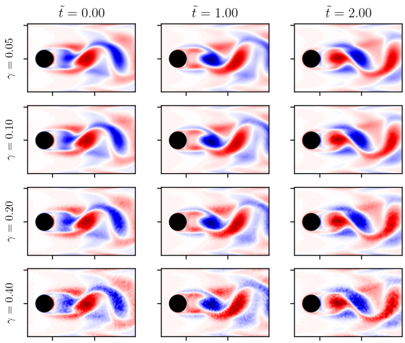
Corrupted vorticity snapshots.

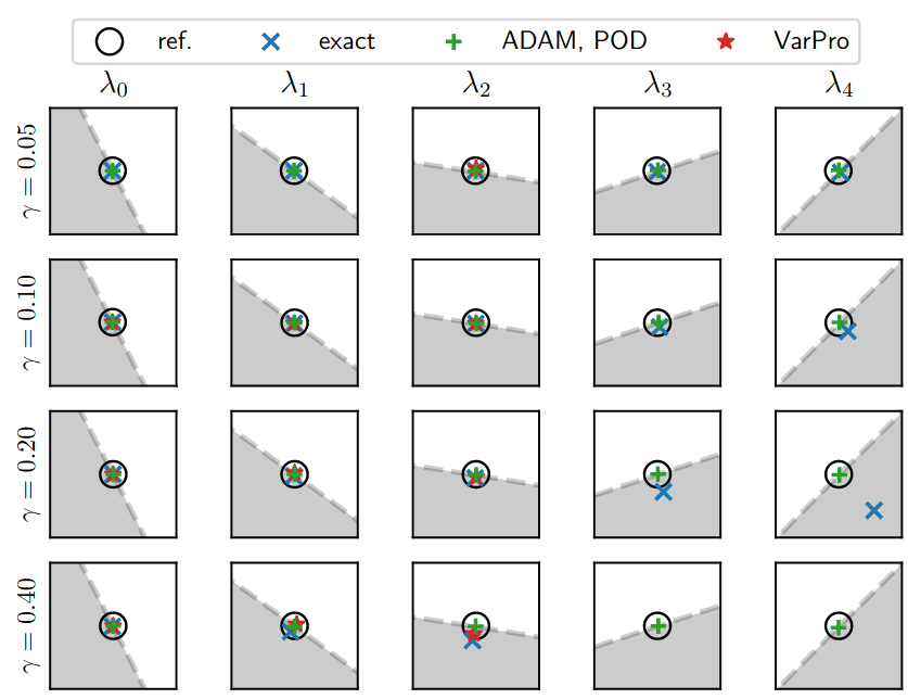
Dominant DMD eigenvalues for various noise levels.