Mathematical model

generic convection-diffusion-equation

What are the in individual terms in transient heat conduction?

What are the in individual terms in a chemically reacting flow?

What is missing to be able to solve the equations?

Mathematical problem considered in this lecture.

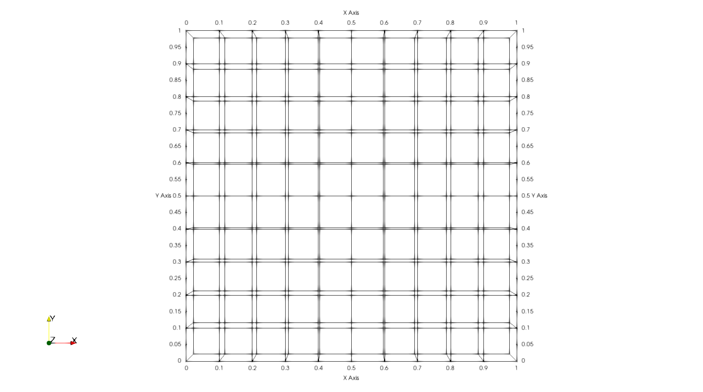
The finite volume mesh

Meshing: subdivide domain into a finite number of discrete elements (control volumes)

Lecture/notebook simplifications:

• structured, Cartesian mesh
• cell-centered variable arrangement

5x5 mesh with grading in $x$.

A class to store the mesh properties

class Mesh(object):
	def __init__(self, L_x, L_y, N_x, N_y, grad_x, grad_y):
		# snip
		self.dx = self._compute_cell_width(L_x, N_x, grad_x)
		self.dy = self._compute_cell_width(L_y, N_y, grad_y)
		self.x = pt.cumsum(self.dx, 0) - self.dx * 0.5
		self.y = pt.cumsum(self.dy, 0) - self.dy * 0.5
	# snip
	def cell_id(self, i, j) -> int:
		return self.N_x * j + i
				

Python intermezzo: (unit) testing

mesh = Mesh(1.0, 1.0, 5, 5, 1.0, 1.0)
assert pt.allclose(mesh.x, pt.linspace(0.1, 0.9, 5))
mesh = Mesh(1.0, 1.0, 5, 5, 2.0, 1.0)
assert pt.isclose(2.0*mesh.dx[0], mesh.dx[-1])
						

A class to store fields and boundary conditions

class VolScalarField(object):
	def __init__(self, mesh, name, value, bc):
		# snip	
	def visualize(self):
		# snip
	def __equal__(self, other):
		return self is other
					

Python intermezzo: equality

# test one
a = [1, 2, 3]
b = a
print(a is b, a == b)
# output?
...
# test two
b = a[:]
print(a is b, a == b)
# output?
						

What changes in an unstructured mesh?

Equation discretization part I - diffusion

Equation discretization: transform PDE + BC/IC into a system of linear equations by means of mesh-based finite PDE approximations for each cell

$$ F\left(T, \partial_t T, \nabla T, ...\right) = 0 \rightarrow \mathbf{Ax} = \mathbf{b} $$

What is the shape of the coefficient matrix for a 5x5 mesh?

What is the length of the source vector for a 5x5 mesh?

A class to store the linear system of equations

class FVMatrix(object):
	def __init__(self, matrix, source, field):
		self.matrix = matrix
		self.source = source
		self.field = field

	def __add__(self, other):
		assert self.field == other.field
		return FVMatrix(self.matrix + other.matrix,
						self.source + other.source,
						self.field)
	# snip
						

Gauss theorem applied to diffusion

$$ \mathbf{n}_n = \qquad, \mathbf{n}_s = \qquad, \mathbf{n}_e = \qquad, \mathbf{n}_w = \qquad $$

$$ \int\limits_{\partial V} \left(\lambda \nabla T\right)\cdot \mathbf{n} \mathrm{d}o = \qquad\qquad\qquad\qquad\qquad $$

$$ s:\quad \int\limits_{x_i-\Delta x_i/2}^{x_i+\Delta x_i/2} \lambda \partial_y T|_s \mathrm{d}x \approx \lambda\Delta x_i g_{y,s}\qquad w:\quad\int\limits_{y_j-\Delta y_j/2}^{y_j+\Delta y_j/2} \lambda \partial_x T|_w \mathrm{d}y \approx \lambda\Delta y_i \frac{T_{i, j} - T_{w}}{0.5\Delta x_i} $$

$$ a_p T_{i,j} + a_n T_{i, j+1} + a_s T_{i, j-1} + a_e T_{i+1, j} + a_w T_{i-1, j} = b $$

Refer to the lecture notebook for more details.

Function to construct the diffusion FVMatrix

def fvm_laplace(diffusivity: float, field: VolScalarField) -> FVMatrix:
    dx, dy = field.mesh.dx, field.mesh.dy
    row, col, val = [], [], []
    source = pt.zeros(field.mesh.N_x*field.mesh.N_y)
    def add_east(i, j):
    # snip
    def add_west(i, j):
    # snip
    for i in range(field.mesh.N_x):
        for j in range(field.mesh.N_y):
            a_e, b_e = add_east(i, j)
            a_w, b_w = add_west(i, j)
            a_n, b_n = add_north(i, j)
            a_s, b_s = add_south(i, j)
            add_center(i, j, (a_e, a_w, a_n, a_s))
            add_source(i, j, (b_e, b_w, b_n, b_s))
        
    return FVMatrix(pt.sparse_coo_tensor([row, col], val),
                    source, field)
						

Combining domain and equation discretization

mesh = Mesh(1.0, 1.0, 5, 5, 1.0, 1.0)
bc = {
    "left" : ("fixedValue", 2.0),
    "right" : ("fixedGradient", -2.0),
    "top" : ("fixedValue", 0.0),
    "bottom" : ("fixedGradient", -5.0),
}
T = VolScalarField(mesh, "T", 0.0, bc)
matrix = fvm_laplace(1.0, T)
						

Coefficient matrix and source vector; blue coeff. are negative; coeff. scaled by absolute value.

Solving a sparse linear system of equations

linear system with two equations and two unknowns

high school (direct) solution

Is the solution correct?

testing the solution

problem: does not scale to large systems of equations

alternative: (iteratively) guessing the solution

x, y = 0, 0
TOL = 1e-3
res_jacobi = []
for i in range(50):
    x_new = (2 + 2*y) / (-1)
    y_new = (-5 + 2*x) / (-7)
    x, y = x_new, y_new
    res_1 = -1*x - 2*y - 2
    res_2 = -2*x - 7*y + 5
    res_jacobi.append(sqrt(res_1**2 + res_2**2))
    print(f"it. {i+1:d}: x={x:1.4f}, y={y:1.4f}, res={res_jacobi[-1]:1.5f}")
    if res_jacobi[-1] < TOL:
        print(f"Converged after {i+1} iterations.")
        break
						

intermediate solution and residuals

it. 1: x=-2.0000, y=0.7143, res=4.24745
it. 2: x=-3.4286, y=1.2857, res=3.07724
it. 3: x=-4.5714, y=1.6939, res=2.42711
it. 4: x=-5.3878, y=2.0204, res=1.75842
# snip
it. 31: x=-7.9986, y=2.9995, res=0.00096
Converged after 31 iterations.
						

Formalizing the Jacobi algorithm

LDU-addressing for coefficient matrix $\mathbf{A}$

$$ \mathbf{A} = \mathbf{L} + \mathbf{D} + \mathbf{U} $$

$$ \boldsymbol{\phi}^{n} = \mathbf{D}^{-1}\mathbf{b} - \mathbf{D}^{-1} (\mathbf{L}+\mathbf{U}) \boldsymbol{\phi}^{n-1} $$

residual in vector-matrix-notation

$$ r^n = |\mathbf{b}-\mathbf{A}\boldsymbol{\phi}^n| $$

more effective updates

x, y = 0, 0
res_gauss_seidel = []
for i in range(50):
	x = (2 + 2*y) / (-1)
	y = (-5 + 2*x) / (-7)
	res_1 = -1*x - 2*y - 2
	res_2 = -2*x - 7*y + 5
	res_gauss_seidel.append(sqrt(res_1**2 + res_2**2))
	print(f"it. {i+1:d}: x={x:1.4f}, y={y:1.4f}, res={res_gauss_seidel[-1]:1.5f}")
	if res_gauss_seidel[-1] < TOL:
		print(f"Converged after {i+1} iterations.")
		break
						

intermediate solution and residuals

it. 1: x=-2.0000, y=1.2857, res=2.57143
it. 2: x=-4.5714, y=2.0204, res=1.46939
it. 3: x=-6.0408, y=2.4402, res=0.83965
it. 4: x=-6.8805, y=2.6801, res=0.47980
# snip
it. 16: x=-7.9986, y=2.9996, res=0.00058
Converged after 16 iterations.
						

Gauss-Seidel vs. Jacobi method.

Formalizing the Gauss-Seidel algorithm

Gauss-Seidel algorithm using LDU-addressing

$$ \mathbf{D}\boldsymbol{\phi}^{n} = \mathbf{b} - \mathbf{L} \boldsymbol{\phi}^{n} - \mathbf{U} \boldsymbol{\phi}^{n-1} $$

$$ \boldsymbol{\phi}^{n} = (\mathbf{D} + \mathbf{L})^{-1} \mathbf{b} - (\mathbf{D} + \mathbf{L})^{-1} \mathbf{U} \boldsymbol{\phi}^{n-1} $$

Avoiding to store zeros: sparse matrices/tensors

1. store non-zero values in a 1D array
2. store row ids of non-zero values in a 1D array
3. store column ids non-zeros values in a 1D array

# sparse tensor in PyTorch
i = [[0, 1, 1],
     [2, 0, 2]]
v =  [3, 4, 5]
s = torch.sparse_coo_tensor(i, v, (2, 3))
s.to_dense()
# output
tensor([[0, 0, 3],
        [4, 0, 5]])

						

Memory requirement of dense and sparse matrices.

def gauss_seidel(A, b, x, tol=1.0e-6, max_iter=1000):
    res_iter = []
    for it in range(max_iter):
        for i in range(x.shape[0]):
            row_sum = 0.0
            for row, col in zip(*A._indices()):
                if row == i and col != i:
                    row_sum += (A[row, col] * x[col]).item()
            x[i] = (b[i] - row_sum) / A[i, i]
        res_iter.append(pt.linalg.norm(b - A.mv(x)).item())
        if res_iter[-1] < tol:
            # snip
						

Implementation of a simple Gauss-Seidel solver.
More efficient: LDU addressing.

Putting it all together

mesh = Mesh(1.0, 1.0, 5, 5, 1.0, 1.0)
bc = {
	"left" : ("fixedValue", 2.0),
	"right" : ("fixedGradient", -2.0),
	"top" : ("fixedValue", 0.0),
	"bottom" : ("fixedGradient", -5.0),
}
T = VolScalarField(mesh, "T", 0.0, bc)
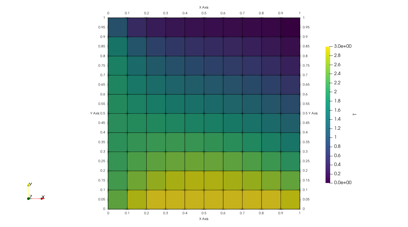
matrix = fvm_laplace(0.1, T)

Tsol = gauss_seidel(matrix.matrix, matrix.source, matrix.field.internal_field.flatten(), tol=1.0e-2)
T = VolScalarField(mesh, "T", Tsol.reshape(5, 5), bc)
						

Cell-centered solution.

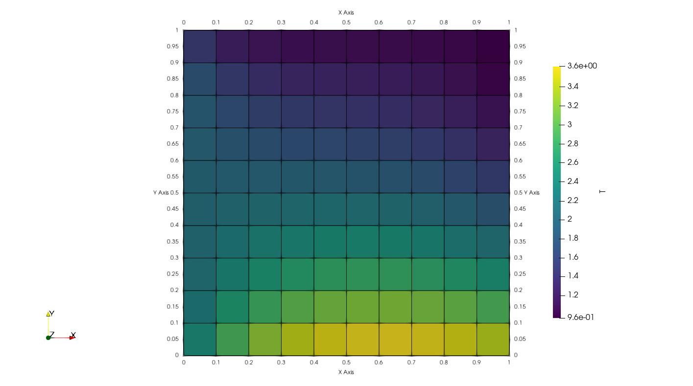
Refined cell-centered solution.

Influence of refinement on convergence.

Linear solvers in CFD are typically iterative

advantages of iterative solvers

• low memory usage
• low computational cost

disadvantages: less robust

Equation discretization part II - convection

Gauss theorem applied to convection

$$ \int\limits_{\partial V} \mathbf{u} T \cdot \mathbf{n} \mathrm{d}o = \qquad\qquad\qquad\qquad\qquad $$

Power law with $n=2$ (source):

$$ \psi = 2 Axy $$ $$ \mathbf{u}(x,y) = (\partial_y \psi, -\partial_x \psi)^T = (2Ax, -2Ay)^T $$

Stream function $\psi = 2 Axy$ and velocity vector $\mathbf{u}(x,y) = (2Ax, -2Ay)^T$.

Velocity vectors in the cell centers and on the surface.

A field type for surface vector fields

class SurfaceVectorField(object):
    def __init__(self, mesh, name, value_x, value_y):
        self.mesh = mesh
        self.name = name
        self.surface_field_x = pt.ones((mesh.N_x + 1, mesh.N_y)) * value_x
        self.surface_field_y = pt.ones((mesh.N_x, mesh.N_y + 1)) * value_y

    def x(self):
        return self.surface_field_x

    def y(self):
        return self.surface_field_y
	# snip
							

$$ s:\quad \int\limits_{x_i-\Delta x_i/2}^{x_i+\Delta x_i/2} u_y T|_s \mathrm{d}x \approx u_{y,s}\Delta x_i (T_{i,j}-0.5 g_{y,s} \Delta y_j)\qquad w:\quad\int\limits_{y_j-\Delta y_j/2}^{y_j+\Delta y_j/2} u_x T|_w \mathrm{d}y \approx u_{x,w}\Delta y_j T_w $$

Function to construct the convection FVMatrix

def fvm_div(vel: SurfaceVectorField,
			field: VolScalarField) -> FVMatrix:
    # snip
    return FVMatrix(pt.sparse_coo_tensor([row, col], val),
                    source, field)
							

Combining domain and equation discretization

mesh = Mesh(1.0, 1.0, 5, 5, 1.0, 1.0)
vel = create_surface_velocity_field(mesh, 1.0)
bc = {
    "left" : ("fixedValue", 2.0),
    "right" : ("fixedGradient", -2.0),
    "top" : ("fixedValue", 1.0),
    "bottom" : ("fixedGradient", -5.0),
}
T = VolScalarField(mesh, "T", 0.0, bc)
matrix = fvm_div(vel, T)
				

Coefficient matrix and source vector; blue coeff. are negative; coeff. scaled by absolute value.

Putting it all together

mesh = Mesh(1.0, 1.0, 10, 10, 1.0, 1.0)
vel = create_surface_velocity_field(mesh, 0.05)
bc = {
    "left" : ("fixedValue", 2.0),
    "right" : ("fixedGradient", -2.0),
    "top" : ("fixedValue", 1.0),
    "bottom" : ("fixedGradient", -5.0),
}
T = VolScalarField(mesh, "T", 0.0, bc)
pde = fvm_div(vel, T) - fvm_laplace(0.1, T)

Tsol, res_coarse = gauss_seidel(
	pde.matrix, pde.source,
	pde.field.internal_field.flatten(),
	tol=1.0e-6
)
T = VolScalarField(mesh, "T", Tsol.reshape(10, 10), bc)
							

Solution converged to $res=9.53\times 10^{-7}$ in 358 iterations.

What could happen if the molecular diffusivity is decreased?

How does a $\partial_t T$ term alter the LSE?

How do I know if the solution is trustworthy?

The FVM in OpenFOAM

Goal: reproduce simulation results in OpenFOAM

$\rightarrow$ test_cases/corner_flow

Instructions provided in the lecture notebook.

output of tree -L 3

├── 0
│   ├── T
│   └── U
├── 0.org
│   ├── T
│   └── U
├── 1
│   ├── phi
│   ├── T
│   └── U
├── Allclean
├── Allrun
├── constant
│   ├── polyMesh
│   │   ├── boundary
│   │   ├── faces
│   │   ├── neighbour
│   │   ├── owner
│   │   └── points
│   └── transportProperties
├── log.blockMesh
├── log.scalarTransportFoam
├── log.setExprFields
├── post.foam
└── system
    ├── blockMeshDict
    ├── controlDict
    ├── fvSchemes
    ├── fvSolution
    └── setExprFieldsDict
					

system/blockMeshDict

scale   1.0;

vertices
(
    (0 0 0)
    (1 0 0)
    (1 1 0)
    (0 1 0)
    (0 0 0.1)
    (1 0 0.1)
    (1 1 0.1)
    (0 1 0.1)
);

blocks
(
    hex (0 1 2 3 4 5 6 7) (10 10 1) simpleGrading (1 1 1)
);

edges
(
);

boundary
(
    top
    {
        type patch;
        faces
        (
            (3 7 6 2)
        );
    }
    bottom
    {
        type wall;
        faces
        (
            (1 5 4 0)
        );
    }
    right
    {
        type patch;
        faces
        (
            (2 6 5 1)
        );
    }
    left
    {
        type wall;
        faces
        (
            (0 4 7 3)
        );
    }
    frontAndBack
    {
        type empty;
        faces
        (
            (0 3 2 1)
            (4 5 6 7)
        );
    }
);
							

OpenFOAM mesh created by blockMesh.

system/exprFieldsDict

expressions
(
    U
    {
        field       U;
        dimensions  [0 1 -1 0 0 0 0];

        variables
        (
            "A = 0.05"
        );

        expression
        #{
            vector (2*A*pos().x(), -2*A*pos().y(), 0.0 )
        #};
    }
);
							

Velocity field initialized with setExprFields.

0.org/T

dimensions      [0 0 0 1 0 0 0];

internalField   uniform 0;

boundaryField
{
    top
    {
        type            fixedValue;
        value           uniform 1.0;
    }

    bottom
    {
        type            fixedGradient;
        gradient        uniform 5.0;
    }

    right
    {
        type            fixedGradient;
        gradient        uniform -2.0;
    }

    left
    {
        type            fixedValue;
        value           uniform 2.0;
    }

    frontAndBack
    {
        type            empty;
    }
}
							

constant/transportProperties

DT              0.1;
				

system/fvSchemes

ddtSchemes
{
    default         steadyState;
}

gradSchemes
{
    default         Gauss linear;
}

divSchemes
{
    default         none;
    div(phi,T)      Gauss linear;
}

laplacianSchemes
{
    default         none;
    laplacian(DT,T) Gauss linear orthogonal;
}
							

system/fvSolution

solvers
{
    T
    {
        solver          smoothSolver;
        smoother        GaussSeidel;
        tolerance       1e-06;
        relTol          0.0;
    }
}
							

Compare the source code of scalarTransportFoam with the Python implementation.

How can I test the setup for pure diffusion?

How can I test the setup for pure convection?

OpenFOAM solution for pure diffusion.

Python solution for pure diffusion.

Solution converged to $res=9.75\times 10^{-7}$ in 364 iterations.

Python solution for convection and diffusion.

The FVM in Basilisk

A minimal list of keywords and properties

• adaptive quadtree/octree meshes
• 2nd order FVM (space and time)
• geometric convective transport (VoF)
• very accurate approximation of surface tension

$\rightarrow$ more information at basilisk.fr

Axis-symmetric rise of a spherical-cap bubble.

Check this example for 3D simulations.