Scale-up approach

Gas-liquid reactors

micro reactor
size: millimeter
source: SPP 1740

prediction of

• mass transfer
• enhancement
• mixing
• conversion
• selectivity
• yield
• ...

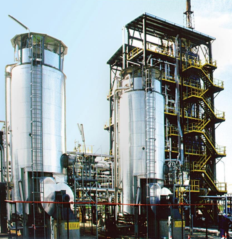
bubble column reactor
size: meter
source: R. M. Raimundo, ENI

Scale-up modeling approach for bubble columns:

• below continuum scale ...
• boundary layers at bubbles ($\mu m$)
• resolved individual bubbles ($mm$)
• bubbles as point particles ($cm$)
• gas-liquid mixture ($m$)

How to transfer information between scales?

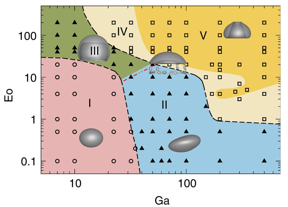
Source: M. K. Tripathi et al. 2015, figure 1.

Potential issues:

• Criterion for the boundaries?
• How to deploy?
• Higher dimensions?
• ...

Potential solution:
supervised learning

Forces acting on a rising bubble

Why does a bubble rise?

1. surface tension forces
2. viscous forces
3. buoyancy forces
4. inertia forces
5. more than one force

What limits the rise velocity?

1. surface tension forces
2. viscous forces
3. buoyancy forces
4. inertia forces
5. more than one force

Why are "small" bubbles spherical/ellipsoidal?

1. surface tension forces
2. viscous forces
3. buoyancy forces
4. inertia forces
5. more than one force

Eötvös or Bond number

$$ Eo = \frac{\text{buoyancy force}}{\text{surface tension force}} = \frac{g\rho_l d_b^2}{\sigma} $$

$\rho_l$ - density liquid, $g$ - gravity, $d_b$ - diameter, $\sigma$ - surface tension

Tells us how strong the deformation is going to be.

Galilei number

$$ Ga = \frac{\text{inertia force}}{\text{viscous force}}\times\sqrt{\frac{\text{buoyancy force}}{\text{inertia force}}} = \frac{\sqrt{gd_b^3}}{\nu_l} $$

$\nu_l$ - kinematic liquid viscosity

Tells us how stable/unstable the rise is going to be.

Source: M. K. Tripathi et al. 2015, figure 1.

Loading, inspecting, and preparing the data

Source: M. K. Tripathi et al. 2015, figure 1.

Data extraction with Engauge Digitizer

• take screenshot of graph/figure
• load screenshot in digitizer
• set origin, axes, and scale
• select markers or lines
• extract to (csv) file

Publish your data (if you can)!

Loading and processing the data.

data_path = "../datasets/path_shape_regimes/"
regimes = ["I", "II", "III", "IV", "V"]
raw_data_files = [f"regime_{regime}.csv" for regime in regimes]
files = [pd.read_csv(data_path + file_name, header=0, names=["Ga", "Eo"]) for file_name in raw_data_files]
for data, regime in zip(files, regimes):
    data["regime"] = regime
data = pd.concat(files, ignore_index=True)
data.sample(5)
# output
Ga	Eo	regime
22.6060	40.557	III
50.0910	39.896	V
6.9836	51.882	III
518.2900	19.694	V
101.0630	19.373	IV
						

Raw extracted data.

$Ga$ and $Eo$ histograms of raw data.

Data transformed using logarithm and $[-1, 1]$ scaling.

$\tilde{Ga}$ and $\tilde{Eo}$ histograms of transformed data.

Adding an ordinal label representation.

# creating an ordinal representation
logData["ordinal"] = 0.0
for i, r in enumerate(regimes):
    logData.ordinal.mask(logData.regime == r, float(i), inplace=True)
						

Binary classification

Goal: distinguish between region I and II.

Only regions I and II

$ \tilde{Ga} = \mathrm{scale}(log(Ga)) $, $ \tilde{Eo} = \mathrm{scale}(log(Eo)) $

$$ z(\tilde{Ga}, \tilde{Eo}) = w_1\tilde{Ga} + w_2\tilde{Eo} + b $$

$$ H(z (\tilde{Ga}, \tilde{Eo})) = \left\{\begin{array}{lr} 0, & \text{if } z \leq 0\\ 1, & \text{if } z \gt 0 \end{array}\right. $$

Variation of weight for $\tilde{Ga}$.

Variation of weight for $\tilde{Eo}$.

Variation of weight for bias $b$.

Heaviside function applied to $z(\tilde{Ga} , \tilde{Eo})$.

Compact notation

Linearly weighted inputs $$ z_i=z(\mathrm{x}_i)=\sum\limits_{j=1}^{N_f}w_jx_{ij} $$

with $$ \mathbf{x}_i = \left[ \tilde{Ga}_i, \tilde{Eo}_i, 1 \right],\quad \mathbf{w} = \left[ w_1, w_2, b \right]^T $$

Binary encoding

True label: $$ y_i = \left\{\begin{array}{lr} 0, & \text{for region I }\\ 1, & \text{for region II} \end{array}\right. $$

Predicted label: $$ \hat{y}_i = H(z_i) = \left\{\begin{array}{lr} 0, & \text{if } z_i \leq 0\\ 1, & \text{if } z_i \gt 0 \end{array}\right. $$

Loss function

The term in parenthesis can take on the values
$1$, $0$, or $-1$.

Gradient decent

Simple update rule for the weights $$ \mathbf{w}^{n+1} = \mathbf{w}^n - l_r \frac{\partial L(\mathbf{w})}{\partial \mathbf{w}} = \begin{pmatrix}w_1^n\\ w_2^n\\ b^n \end{pmatrix} + l_r \sum\limits_{i=1}^N \left(y_i - \hat{y}_i^n \right) \begin{pmatrix}\tilde{Ga}_i\\ \tilde{Eo}_i\\ 1 \end{pmatrix} $$

$n$ - current iteration, $l_r$ - learning rate

Implementation of the perceptron algorithm.

class Perceptron(object):
    def __init__(self, n_weights: int):
        self._p = pt.rand(n_weights)*2.0 - 1.0

    def _loss(self, X: pt.Tensor, y: pt.Tensor) -> pt.Tensor:
        return 0.5 * pt.sum((y - self.predict(X))**2)

    def _loss_gradient(self, X: pt.Tensor, y: pt.Tensor) -> pt.Tensor:
        delta = y - self.predict(X)
        return -pt.cat((X, pt.ones(X.shape[0]).unsqueeze(-1)), dim=-1).T.mv(delta)

    def train(self, X: pt.Tensor, y: pt.Tensor, epochs: int=500,
              lr: float=0.01, tol: float=1.0e-6) -> List[float]:
        loss = []
        for e in range(epochs):
            self._p -= lr*self._loss_gradient(X, y)
            loss.append(self._loss(X, y).item())
            if loss[-1] < tol:
                print(f"Converged after {e+1} epochs.")
                return loss
        print(f"Training did not converge within {epochs} epochs")
        print(f"Final loss: {loss[-1]:2.3f}")
        return loss

    def predict(self, X: pt.Tensor):
        weighted_sum = X.mv(self._p[:-1]) + self._p[-1]
        return pt.heaviside(weighted_sum, pt.tensor(0.0))
						

Perceptron learning rule - loss over epochs.

Perceptron algorithm - weighted sum of inputs and prediction.

Guaranteed convergence (zero loss)?

1. yes
2. no
3. data dependent

Conditional probabilities

speak: probability $p$ of the event $y=1$ given $\mathrm{x}$

model predicts class probability instead of class!

What is the expected value of $p(y=1 | \mathrm{x})$ for points far in region II?

1. close to zero
2. about 0.5
3. close to one

What is the expected value of $p(y=1 | \mathrm{x})$ for points far in region I?

1. close to zero
2. about 0.5
3. close to one

What is the expected value of $p(y=1 | \mathrm{x})$ for points close to the decision boundary?

1. close to zero
2. about 0.5
3. close to one

What is the expected value of $p(y=0 | \mathrm{x})$ for points far in region I?

1. close to zero
2. about 0.5
3. close to one

How to convert $z(\mathrm{x})$ to a probability?

1. sinus: $\mathrm{sin}(z)$
2. hyperbolic tangents: $\mathrm{tanh}(z)$
3. sigmoid: $\sigma(z)$

Sigmoid function $\sigma = 1 / (1+\mathrm{exp}(-z))$.

Probabilities $p(II|\tilde{Ga},\tilde{Eo}) = \sigma (z(\tilde{Ga},\tilde{Eo}))$.

Joint probabilities - likelihood function

principle of maximum likelihood

Which of the following is equivalent to $l(\mathbf{w}) = \prod\limits_i^{N_s} p_i(y_i | \mathbf{x}_i)$?

1. $$ \prod\limits_i^{N_s} \left[ y_i^{\hat{y}_i} (1-y_i)^{(1-\hat{y}_i)}\right] $$
2. $$ \prod\limits_i^{N_s} \left[ \hat{y}_i^{y_i} (1-\hat{y}_i)^{(1-y_i)}\right] $$

Log-likelihood and binary cross entropy

$$ \mathrm{ln}(l(\mathbf{w})) = \sum\limits_{i=1}^{N_s} y_i \mathrm{ln}(\hat{y}_i) + (1-y_i) \mathrm{ln}(1-\hat{y}_i) $$

$$ L(\mathbf{w}) = -\frac{1}{N_s}\sum\limits_{i=1}^{N_s} y_i \mathrm{ln}(\hat{y}_i) + (1-y_i) \mathrm{ln}(1-\hat{y}_i) $$

Implementation of logistic regression.

class LogisticRegression(object):
    def __init__(self, n_weights):
        self._p = pt.rand(n_weights)*2.0 - 1.0

    def _joint_probability(self, X: pt.Tensor, y: pt.Tensor) -> pt.Tensor:
        probs = self.probability(X)
        joint = pt.pow(probs, y) * pt.pow(1.0-probs, 1-y)
        return pt.prod(joint)

    def _loss(self, X: pt.Tensor, y: pt.Tensor) -> pt.Tensor:
        probs = self.probability(X)
        entropy = y*pt.log(probs+1.0e-6) + (1-y)*pt.log(1.0-probs+1.0e-6)
        return -entropy.mean()

    def _loss_gradient(self, X: pt.Tensor, y: pt.Tensor) -> pt.Tensor:
        delta = y - self.probability(X)
        grad = pt.cat((X, pt.ones(X.shape[0]).unsqueeze(-1)), dim=-1) * delta.unsqueeze(-1)
        return -grad.mean(dim=0)

    def train(self, X: pt.Tensor, y: pt.Tensor, epochs: int=10000,
        # snip - see perceptron

    def probability(self, X: pt.Tensor) -> pt.Tensor:
        weighted_sum = X.mv(self._p[:-1]) + self._p[-1]
        return pt.sigmoid(weighted_sum)

    def predict(self, X: pt.Tensor) -> pt.Tensor:
        return pt.heaviside(self.probability(X)-0.5, pt.tensor(0.0))
						

Binary cross entropy vs. epochs.

Landscape around the optima of binary cross entropy and joint probability.

Probability and prediction with logistic regression.

New goal: separate regime I from II and III.

Logistic regression classifiers separating regions I-II and I-III.

Training of two logistic regressors.

	combined_prob = pt.sigmoid(
	  0.9*model_I_II.probability(pt.stack((xx.flatten(), yy.flatten())).T)
	+ 0.9*model_I_III.probability(pt.stack((xx.flatten(), yy.flatten())).T)
	- 0.5
	)
	combined_prediction = pt.heaviside(combined_prob - 0.5, pt.tensor(0.0))
						

Combination of two logistic regression classifiers.

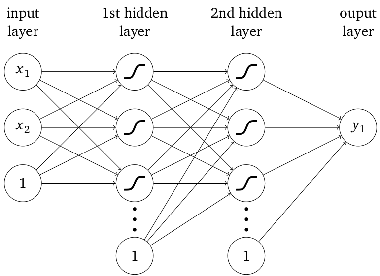
Generic neural network with fully connected layers.

Multi-class classification

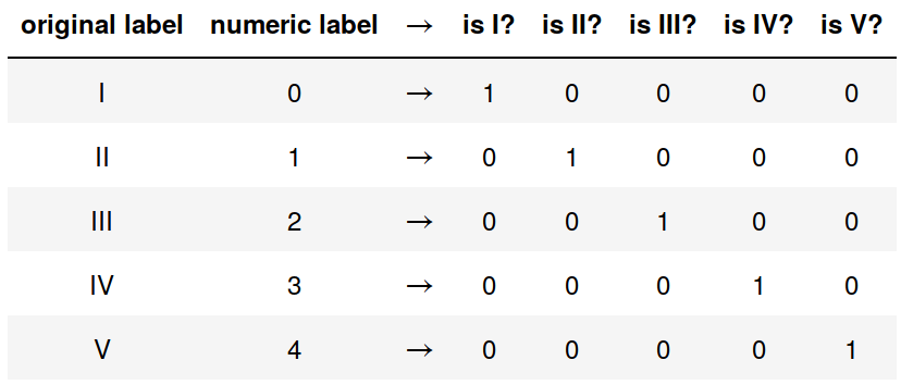
One hot encoding of path regimes.

What is the length of the label vector if we have 10 classes (regimes)?

1. 1
2. 2
3. 5
4. 10

What does the label vector look like if we have 4 classes and the true label is class 3 / regime 3 (start counting from 1)?

1. $\mathbf{y}_i = \left[ 1, 0, 0, 0 \right]^T$
2. $\mathbf{y}_i = \left[ 0, 0, 1, 0 \right]^T$
3. $\mathbf{y}_i = \left[ 1, 0, 1, 0 \right]^T$
4. $\mathbf{y}_i = \left[ 0, 0, 3, 0 \right]^T$

Softmax function and categorical cross entropy for $K$ classes:

$$ p(y_{j}=1 | \mathbf{x}) = \frac{e^{z_{j}}}{\sum_{j=0}^{K-1} e^{z_{j}}} $$

$$ L(\mathbf{w}) = -\frac{1}{N} \sum\limits_{i=1}^{N_s}\sum\limits_{j=0}^{K-1} y_{ij} \mathrm{ln}\left( \hat{y}_{ij} \right) $$

What is a likely/possible prediction if the true class is 3 (start counting from 1)?

1. $\hat{\mathbf{y}}_i = \left[ 0.1, 0, 0.9, 0.1 \right]^T$
2. $\hat{\mathbf{y}}_i = \left[ 1, 0, 0, 0 \right]^T$
3. $\hat{\mathbf{y}}_i = \left[ 0, 0.02, 0.95, 0.03 \right]^T$
4. $\hat{\mathbf{y}}_i = \left[ 0, 0, 3, 0 \right]^T$

Neural network classification model.

n_features, n_classes, n_neurons = 2, 5, 50
regime_model = pt.nn.Sequential(
    pt.nn.Linear(n_features, n_neurons),
    pt.nn.Tanh(),
    pt.nn.Linear(n_neurons, n_neurons),
    pt.nn.Tanh(),
    pt.nn.Linear(n_neurons, n_classes)
)
						

Training loop definition.

dataset = pt.utils.data.TensorDataset(
    pt.tensor(logData[["Ga", "Eo"]].values, dtype=pt.float32),
    pt.tensor(logData.ordinal.values, dtype=pt.int64)
)
train_size = int(0.9*len(dataset))
val_size = len(dataset) - train_size
train_dataset, val_dataset = pt.utils.data.random_split(dataset, (train_size, val_size))
train_loader = pt.utils.data.DataLoader(train_dataset, batch_size=len(train_dataset), shuffle=True)
val_loader = pt.utils.data.DataLoader(val_dataset, batch_size=len(val_dataset))

results = train_model(regime_model, pt.nn.CrossEntropyLoss(), train_loader, val_loader,
                      epochs=1000, optimizer=optimizer)
						

Categorical cross entropy vs. epochs.

Prediction of classification network.